Why LLM mathematics comes after probability and tensors
In the previous sections, we studied:
$$ \text{vectors},\quad \text{matrices},\quad \text{tensors}, $$then probability distributions, Gaussian noise, Markov chains, stochastic processes, and diffusion models.
Large language models use all of these ideas.
An LLM is not just a “text generator.” Mathematically, it is a large parameterized probability model over sequences of tokens.
A sentence becomes a sequence:
$$ x_1,x_2,\dots,x_T. $$Each token becomes a vector:
$$ e_t \in \mathbb{R}^{d_{\text{model}}}. $$A full sequence becomes a matrix:
$$ X \in \mathbb{R}^{T \times d_{\text{model}}}. $$A batch becomes a tensor:
$$ X \in \mathbb{R}^{B \times T \times d_{\text{model}}}. $$A transformer maps this tensor into another tensor, and the final layer produces a probability distribution over the next token.
The key mathematical goal is:
$$ p_\theta(x_{t+1}\mid x_1,\dots,x_t). $$That means:
given previous tokens, predict the probability distribution of the next token.
Modern LLMs are built on the Transformer architecture, introduced in Attention Is All You Need, which replaced recurrence and convolution with attention mechanisms and enabled much more parallel training. (arXiv)
Part I — Text as mathematics
From words to numbers
A computer cannot directly process the sentence:
Mathematics is the language of AI.
It must first convert text into numbers.
A simple but bad idea is to assign one number to each word:
| Word | Number |
|---|---|
| Mathematics | 1 |
| is | 2 |
| the | 3 |
| language | 4 |
| of | 5 |
| AI | 6 |
Then the sentence becomes:
$$ [1,2,3,4,5,6]. $$But this has a problem.
The number 6 is not “larger” than the number 1 in any meaningful semantic way. These numbers are just identifiers.
So we need a better representation.
The usual pipeline is:
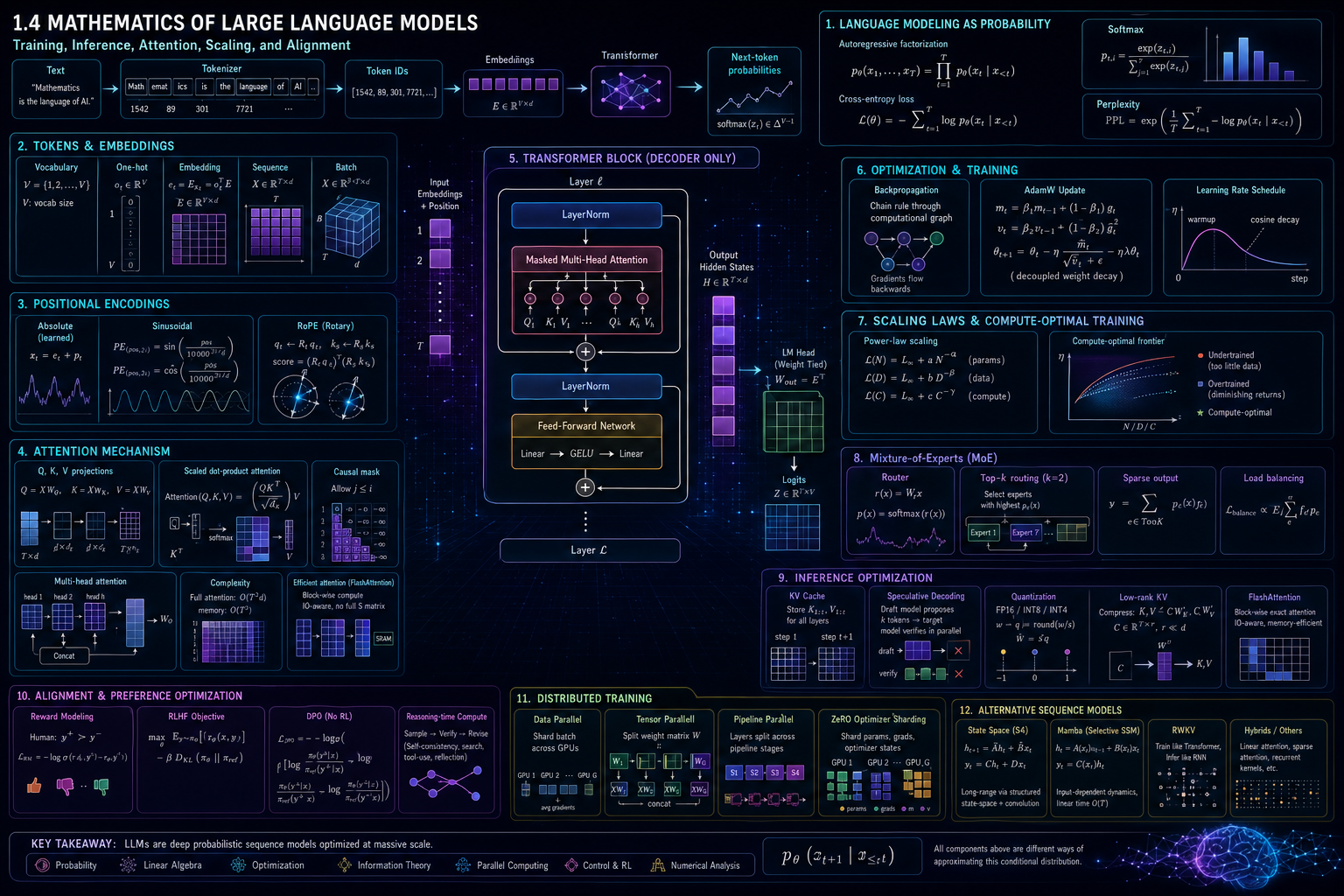
$$ \text{text} \longrightarrow \text{tokens} \longrightarrow \text{token IDs} \longrightarrow \text{embedding vectors} \longrightarrow \text{transformer computation} \longrightarrow \text{next-token probabilities}. $$Tokens
A token is a unit of text used by the model.
A token may be:
- a word,
- part of a word,
- punctuation,
- a space,
- a byte sequence,
- or another subword unit.
For example, the word:
mathematics
may be one token in one tokenizer, but split into subwords in another tokenizer.
Subword tokenization became important because natural language has rare words, new words, names, code symbols, numbers, and multilingual forms. BPE-based subword modeling was introduced for neural machine translation to handle rare and unknown words by encoding them as subword units rather than relying on a fixed word vocabulary. (arXiv)
SentencePiece later provided a language-independent tokenizer/detokenizer that can train directly from raw sentences, without assuming pre-tokenized word sequences. (arXiv)
Vocabulary
Let the vocabulary be:
$$ \mathcal{V} {}={} {1,2,\dots,V}. $$Here:
- \(V\) is the vocabulary size,
- each token is represented by an integer ID,
- \(x_t \in \mathcal{V}\) is the token at position \(t\).
For example:
$$ x = [x_1,x_2,x_3,x_4] {}={} [1542,89,301,7721]. $$This is a sequence of token IDs.
The model does not yet understand meaning. These are still just integers.
One-hot representation
A token ID can be represented as a one-hot vector.
If:
$$ V=5 $$and the token ID is:
$$ x_t=3, $$then the one-hot vector is:
$$ o_t = \begin{bmatrix} 0\ 0\ 1\ 0\ 0 \end{bmatrix}. $$So:
$$ o_t \in \mathbb{R}^{V}. $$But one-hot vectors are huge and sparse.
If:
$$ V=100{,}000, $$then every token would be a 100,000-dimensional vector with only one nonzero entry.
So LLMs use embeddings.
Embedding matrix
An embedding matrix is:
$$ E \in \mathbb{R}^{V \times d}. $$Here:
- \(V\) is vocabulary size,
- \(d=d_{\text{model}}\) is embedding dimension.
Each row of \(E\) is a learned vector for one token.
If token \(x_t\) has ID \(i\), then its embedding is:
$$ e_t = E_i. $$Equivalently, using a one-hot vector:
$$ e_t = o_t^\top E. $$Shape-wise:
$$ (1\times V)(V\times d)=1\times d. $$So a token ID becomes a dense vector:
$$ e_t \in \mathbb{R}^{d}. $$This is the first major mathematical transformation:
$$ \text{discrete token} \longrightarrow \text{continuous vector}. $$Sequence embedding matrix
For a sequence of \(T\) tokens:
$$ x_1,x_2,\dots,x_T, $$we get embeddings:
$$ e_1,e_2,\dots,e_T. $$Stack them row by row:
$$ X = \begin{bmatrix} e_1^\top\ e_2^\top\ \vdots\ e_T^\top \end{bmatrix} \in \mathbb{R}^{T\times d}. $$For a batch of \(B\) sequences:
$$ X \in \mathbb{R}^{B\times T\times d}. $$This is the tensor that enters the transformer.
Part II — Language modeling as probability
The language-modeling problem
A language model assigns probabilities to token sequences.
Given:
$$ x_1,x_2,\dots,x_T, $$the model wants:
$$ p_\theta(x_1,x_2,\dots,x_T). $$Using the chain rule of probability:
$$ p_\theta(x_1,\dots,x_T) {}={} \prod_{t=1}^{T} p_\theta(x_t\mid x_1,\dots,x_{t-1}). $$This is the central factorization of autoregressive language modeling.
The model predicts each token using the previous tokens.
For example:
$$ p_\theta(\text{`AI''}\mid \text{`Mathematics for''}). $$Autoregressive modeling
An autoregressive model generates tokens one at a time.
At step \(t\), it computes:
$$ p_\theta(x_{t+1}\mid x_1,\dots,x_t). $$Then it chooses or samples the next token.
After generating \(x_{t+1}\), it repeats:
$$ p_\theta(x_{t+2}\mid x_1,\dots,x_t,x_{t+1}). $$So generation is sequential:
$$ x_1 \rightarrow x_2 \rightarrow x_3 \rightarrow \cdots. $$This sequential nature is one reason inference is expensive: generating \(K\) new tokens usually requires \(K\) decoding steps. Speculative decoding papers explicitly identify autoregressive token-by-token decoding as a major latency bottleneck. (arXiv)
Log-likelihood
Suppose the training dataset contains sequences:
$$ \mathcal{D}={x^{(1)},x^{(2)},\dots,x^{(N)}}. $$The likelihood is:
$$ L(\theta) {}={} \prod_{n=1}^{N} p_\theta(x^{(n)}). $$Because products of many probabilities become extremely small, we use log-likelihood:
$$ \log L(\theta) {}={} \sum_{n=1}^{N} \log p_\theta(x^{(n)}). $$For autoregressive models:
$$ \log p_\theta(x^{(n)}) {}={} \sum_{t=1}^{T_n} \log p_\theta(x_t^{(n)}\mid x_{Equivalently, we minimize negative log-likelihood:
$$ \mathcal{L}(\theta) {}={} * \sum_{n=1}^{N} \sum_{t=1}^{T_n} \log p_\theta(x_t^{(n)}\mid x_{The Deep Learning book connects maximum likelihood learning with cross-entropy loss for neural networks. (Deep Learning Book)
Softmax distribution over vocabulary
At each position \(t\), the model outputs logits:
$$ z_t \in \mathbb{R}^{V}. $$Each component \(z_{t,i}\) is a score for token \(i\).
To convert logits into probabilities, use softmax:
$$ p_{t,i} {}={} \frac{\exp(z_{t,i})} {\sum_{j=1}^{V}\exp(z_{t,j})}. $$The output vector is:
$$ p_t = \operatorname{softmax}(z_t) \in \mathbb{R}^{V}. $$It satisfies:
$$ p_{t,i}\geq 0 $$and:
$$ \sum_{i=1}^{V}p_{t,i}=1. $$So softmax turns scores into a probability distribution.
Cross-entropy loss
If the true next token is \(y_t\), then the target distribution is one-hot:
$$ q_{t,i} {}={} \begin{cases} 1, & i=y_t,\ 0, & i\neq y_t. \end{cases} $$The cross-entropy is:
$$ H(q_t,p_t) {}={} -\sum_{i=1}^{V}q_{t,i}\log p_{t,i}. $$Because \(q_t\) is one-hot, this becomes:
$$ H(q_t,p_t) {}={} -\log p_{t,y_t}. $$So for one token, the loss is:
$$ \ell_t {}={} -\log p_\theta(y_t\mid x_{Perplexity
Perplexity is a common language-model evaluation metric.
If the average negative log-likelihood per token is:
$$ \bar{\mathcal{L}} {}={} -\frac{1}{T} \sum_{t=1}^{T} \log p_\theta(x_t\mid x_{Lower perplexity means the model assigns higher probability to the correct tokens.
But perplexity is not the same as human usefulness, reasoning quality, safety, or instruction-following ability.
Part III — The Transformer block
Why transformers changed language modeling
Before transformers, sequence models often used recurrence.
A recurrent model processes tokens one by one:
$$ h_t=f(h_{t-1},x_t). $$This makes training harder to parallelize across sequence positions.
The transformer instead uses attention, allowing all positions in a sequence to interact through matrix operations. The original Transformer paper proposed an architecture based solely on attention mechanisms, dispensing with recurrence and convolution. (arXiv)
Input tensor
For one sequence:
$$ X\in\mathbb{R}^{T\times d}. $$For a batch:
$$ X\in\mathbb{R}^{B\times T\times d}. $$A transformer block maps:
$$ X \mapsto X' $$where:
$$ X'\in\mathbb{R}^{B\times T\times d}. $$So the shape is preserved across blocks.
A stack of \(L\) transformer blocks gives:
$$ X^{(0)} \to X^{(1)} \to \cdots \to X^{(L)}. $$Linear projections: queries, keys, and values
Inside attention, each token vector is projected into three vectors:
$$ q_t = x_t W_Q, $$$$ k_t = x_t W_K, $$$$ v_t = x_t W_V. $$For the whole sequence:
$$ Q=XW_Q, $$$$ K=XW_K, $$$$ V=XW_V. $$If:
$$ X\in\mathbb{R}^{T\times d}, $$and:
$$ W_Q,W_K,W_V\in\mathbb{R}^{d\times d_k}, $$then:
$$ Q,K,V\in\mathbb{R}^{T\times d_k}. $$The names are intuitive:
- query: what this token is looking for,
- key: what this token offers for matching,
- value: information to pass forward.
Dot-product attention
The similarity between token \(i\) and token \(j\) is:
$$ s_{ij}=q_i^\top k_j. $$Stacking all similarities gives:
$$ S=QK^\top. $$Shape-wise:
$$ (T\times d_k)(d_k\times T)=T\times T. $$So:
$$ S\in\mathbb{R}^{T\times T}. $$Each entry \(S_{ij}\) measures how much token \(i\) attends to token \(j\).
Scaled dot-product attention
The transformer uses scaled dot-product attention:
$$ \operatorname{Attention}(Q,K,V) {}={} \operatorname{softmax} \left( \frac{QK^\top}{\sqrt{d_k}} \right)V. $$This is the central formula of transformer mathematics.
The scaling factor:
$$ \frac{1}{\sqrt{d_k}} $$prevents dot products from becoming too large when dimension \(d_k\) is large.
The Transformer paper introduced scaled dot-product attention and multi-head attention as core components of the architecture. (arXiv)
Attention weights
Define:
$$ A= \operatorname{softmax} \left( \frac{QK^\top}{\sqrt{d_k}} \right). $$Then:
$$ A\in\mathbb{R}^{T\times T}. $$Each row sums to 1:
$$ \sum_{j=1}^{T}A_{ij}=1. $$The output is:
$$ O=AV. $$For token \(i\):
$$ o_i {}={} \sum_{j=1}^{T}A_{ij}v_j. $$So attention outputs a weighted average of value vectors.
Causal masking
For language generation, token \(t\) must not see future tokens.
So we use a causal mask.
Without masking, token \(i\) could attend to token \(j>i\), which would leak the answer during training.
The masked attention score is:
$$ \tilde{S}_{ij} {}={} \begin{cases} S_{ij}, & j\leq i,\ -\infty, & j>i. \end{cases} $$Then:
$$ A= \operatorname{softmax} \left( \frac{\tilde{S}}{\sqrt{d_k}} \right). $$This ensures:
$$ A_{ij}=0 \quad \text{for} \quad j>i. $$So each token only attends to itself and previous tokens.
Multi-head attention
Instead of one attention operation, transformers use multiple heads.
For head \(h\):
$$ Q_h=XW_Q^{(h)}, $$$$ K_h=XW_K^{(h)}, $$$$ V_h=XW_V^{(h)}. $$Then:
$$ O_h= \operatorname{Attention}(Q_h,K_h,V_h). $$The heads are concatenated:
$$ O= \operatorname{Concat}(O_1,\dots,O_H)W_O. $$Multi-head attention allows different heads to learn different relationships.
One head may focus on syntax.
Another may focus on long-range references.
Another may focus on local patterns.
Mathematically, each head is a separate learned bilinear similarity mechanism.
Attention complexity
For sequence length \(T\), attention forms:
$$ QK^\top\in\mathbb{R}^{T\times T}. $$So standard attention requires:
$$ O(T^2) $$attention scores.
This is the main long-context bottleneck.
If \(T=4{,}000\), then:
$$ T^2=16{,}000{,}000. $$If \(T=128{,}000\), then:
$$ T^2=16{,}384{,}000{,}000. $$So long-context LLMs require efficient attention algorithms, memory management, KV compression, sparse patterns, or alternative sequence models.
FlashAttention addresses this by computing exact attention with an IO-aware tiled algorithm that reduces memory reads and writes between GPU memory levels. (arXiv)
FlashAttention-2 further improves speed through better work partitioning and parallelism. (arXiv)
Part IV — Positional information
Why position matters
Attention by itself is permutation-invariant.
If we only give the model a bag of token vectors, it does not know which token came first.
For example:
dog bites man
and:
man bites dog
contain the same words but different meanings.
So transformers need positional information.
Absolute positional embeddings
A simple approach is to learn a position embedding matrix:
$$ P\in\mathbb{R}^{T_{\max}\times d}. $$For position \(t\), add:
$$ x_t = e_t+p_t. $$So token identity and position are combined:
$$ X = E_{\text{tokens}} + P_{\text{positions}}. $$Sinusoidal positional encoding
The original Transformer used sinusoidal positional encodings:
$$ PE_{(pos,2i)} {}={} \sin \left( \frac{pos}{10000^{2i/d}} \right), $$$$ PE_{(pos,2i+1)} {}={} \cos \left( \frac{pos}{10000^{2i/d}} \right). $$These provide deterministic position-dependent vectors.
Rotary position embedding
Rotary Position Embedding, or RoPE, applies position-dependent rotations to query and key vectors.
At a high level:
$$ q_t \mapsto R_t q_t, $$$$ k_s \mapsto R_s k_s. $$Then the attention score becomes:
$$ (R_tq_t)^\top(R_sk_s). $$Because rotations interact through relative differences, RoPE naturally introduces relative position information into attention.
The RoFormer paper describes RoPE as encoding absolute position with a rotation matrix while incorporating explicit relative-position dependency in self-attention. (arXiv)
Part V — Normalization, residuals, and feed-forward networks
Residual connections
A transformer block usually uses residual connections.
If a sublayer computes:
$$ F(X), $$then the residual output is:
$$ Y=X+F(X). $$Residual connections help gradients flow through many layers.
They also allow a layer to learn a correction rather than a full transformation.
Layer normalization
Layer normalization normalizes a vector across its feature dimension.
For:
$$ x\in\mathbb{R}^{d}, $$define:
$$ \mu {}={} \frac{1}{d}\sum_{i=1}^{d}x_i, $$$$ \sigma^2 {}={} \frac{1}{d}\sum_{i=1}^{d}(x_i-\mu)^2. $$Then:
$$ \operatorname{LayerNorm}(x) {}={} \gamma \odot \frac{x-\mu}{\sqrt{\sigma^2+\epsilon}} + \beta. $$Here:
- \(\gamma\) is learned scale,
- \(\beta\) is learned shift,
- \(\epsilon\) prevents division by zero.
RMSNorm
RMSNorm removes mean-centering and uses root mean square normalization:
$$ \operatorname{RMS}(x) {}={} \sqrt{ \frac{1}{d} \sum_{i=1}^{d}x_i^2 }. $$Then:
$$ \operatorname{RMSNorm}(x) {}={} \gamma \odot \frac{x}{\operatorname{RMS}(x)+\epsilon}. $$RMSNorm was proposed as a computationally simpler alternative to LayerNorm that keeps rescaling invariance while avoiding recentering. (arXiv)
Feed-forward network
After attention, each token passes through a feed-forward network.
A standard feed-forward block is:
$$ \operatorname{FFN}(x) {}={} W_2\phi(W_1x+b_1)+b_2. $$Here:
- \(W_1\in\mathbb{R}^{d\times d_{\text{ff}}}\),
- \(W_2\in\mathbb{R}^{d_{\text{ff}}\times d}\),
- \(\phi\) is a nonlinear activation.
The feed-forward network is applied independently to each token.
So attention mixes information across positions, while the FFN transforms each token representation.
Gated feed-forward networks
Many modern transformers use gated FFNs.
A common form is:
$$ \operatorname{FFN}(x) {}={} (W_gx \odot \phi(W_ux))W_d. $$Here:
- \(W_g\) produces a gate,
- \(W_u\) produces candidate features,
- \(\odot\) is elementwise multiplication,
- \(W_d\) projects back to model dimension.
This allows the model to control which features pass through.
Part VI — The full decoder-only transformer
One transformer block
A simplified decoder block is:
$$ Y = X + \operatorname{Attention}(\operatorname{Norm}(X)), $$$$ Z = Y + \operatorname{FFN}(\operatorname{Norm}(Y)). $$So each block contains:
- normalization,
- causal self-attention,
- residual connection,
- normalization,
- feed-forward network,
- residual connection.
Stack \(L\) blocks:
$$ X^{(0)} \to X^{(1)} \to \cdots \to X^{(L)}. $$At the end:
$$ H=X^{(L)}. $$The final logits are:
$$ Z=HW_{\text{out}}. $$If:
$$ H\in\mathbb{R}^{T\times d}, $$and:
$$ W_{\text{out}}\in\mathbb{R}^{d\times V}, $$then:
$$ Z\in\mathbb{R}^{T\times V}. $$Each row gives logits for the next-token distribution.
Weight tying
Often the output matrix is tied to the input embedding matrix:
$$ W_{\text{out}}=E^\top. $$If:
$$ E\in\mathbb{R}^{V\times d}, $$then:
$$ E^\top\in\mathbb{R}^{d\times V}. $$This reduces parameters and connects input and output token representations.
Part VII — Backpropagation and optimization
Parameters
Let all model parameters be collected into:
$$ \theta. $$This includes:
- token embeddings,
- attention matrices,
- feed-forward matrices,
- normalization parameters,
- output projection,
- router parameters in MoE models,
- adapter or LoRA parameters if fine-tuning.
Training minimizes:
$$ \mathcal{L}(\theta). $$The mathematical goal is:
$$ \theta^\star {}={} \arg\min_\theta \mathcal{L}(\theta). $$Gradient descent
The gradient is:
$$ \nabla_\theta \mathcal{L}(\theta). $$Gradient descent updates:
$$ \theta_{k+1} {}={} \theta_k - \eta \nabla_\theta \mathcal{L}(\theta_k). $$Here:
- \(\eta\) is learning rate,
- \(k\) is optimization step.
For LLMs, the loss is computed on minibatches.
So we use stochastic gradients:
$$ g_k {}={} \nabla_\theta \mathcal{L}_{\mathcal{B}_k}(\theta_k). $$Backpropagation
Backpropagation applies the chain rule through the computational graph.
For a composition:
$$ y=f(g(h(x))), $$the derivative is:
$$ \frac{dy}{dx} {}={} \frac{dy}{df} \frac{df}{dg} \frac{dg}{dh} \frac{dh}{dx}. $$In matrix form, backpropagation repeatedly multiplies local Jacobians.
For a linear layer:
$$ Y=XW, $$if:
$$ G_Y=\frac{\partial \mathcal{L}}{\partial Y}, $$then:
$$ \frac{\partial \mathcal{L}}{\partial W} {}={} X^\top G_Y, $$and:
$$ \frac{\partial \mathcal{L}}{\partial X} {}={} G_Y W^\top. $$Stanford CS231n notes explicitly derive minibatch backpropagation for a linear layer \(Y=XW\). (CS231n)
Adam optimizer
Adam uses moving averages of gradients and squared gradients.
Given gradient:
$$ g_t=\nabla_\theta \mathcal{L}_t(\theta_t), $$Adam computes:
$$ m_t=\beta_1m_{t-1}+(1-\beta_1)g_t, $$$$ v_t=\beta_2v_{t-1}+(1-\beta_2)g_t^2. $$Bias-corrected estimates are:
$$ \hat{m}_t=\frac{m_t}{1-\beta_1^t}, $$$$ \hat{v}_t=\frac{v_t}{1-\beta_2^t}. $$Then:
$$ \theta_{t+1} {}={} \theta_t - \eta \frac{\hat{m}_t}{\sqrt{\hat{v}_t}+\epsilon}. $$Adam was introduced as a first-order stochastic optimization method using adaptive estimates of lower-order moments. (arXiv)
AdamW
Weight decay penalizes large weights.
A naive \(L^2\) penalty adds:
$$ \lambda |\theta|_2^2 $$to the loss.
AdamW decouples weight decay from the adaptive gradient update.
A simplified AdamW update is:
$$ \theta_{t+1} {}={} \theta_t - \eta \frac{\hat{m}_t}{\sqrt{\hat{v}_t}+\epsilon} - \eta\lambda\theta_t. $$The AdamW paper shows that \(L^2\) regularization and weight decay are not equivalent for adaptive optimizers such as Adam, and proposes decoupled weight decay. (arXiv)
Learning-rate schedules
LLM training often uses a schedule:
- warmup,
- decay,
- sometimes a final constant or cosine tail.
During warmup:
$$ \eta_t {}={} \eta_{\max}\frac{t}{T_{\text{warmup}}}. $$A cosine decay may be:
$$ \eta_t {}={} \eta_{\min} + \frac{1}{2} (\eta_{\max}-\eta_{\min}) \left[ 1+\cos\left(\frac{\pi t}{T}\right) \right]. $$The purpose is to avoid instability early and reduce noise later.
Gradient clipping
If gradients become too large, training may diverge.
Gradient norm clipping uses:
$$ g \leftarrow g\cdot \min \left( 1, \frac{c}{|g|_2} \right). $$If:
$$ |g|_2\leq c, $$nothing changes.
If:
$$ |g|_2>c, $$the gradient is rescaled.
Part VIII — Scaling laws and compute-optimal training
Why scaling laws matter
LLMs are expensive.
We must decide:
- how many parameters,
- how many training tokens,
- how much compute,
- how much data quality filtering,
- how much context length,
- how many experts,
- how many training stages.
Scaling laws try to describe how loss changes as model size, data size, and compute change.
Kaplan et al. found empirical power-law relationships between cross-entropy loss and model size, dataset size, and training compute over large ranges. (arXiv)
Power-law form
A simplified scaling law is:
$$ L(N) {}={} L_\infty + aN^{-\alpha}. $$Here:
- \(L(N)\) is loss,
- \(N\) is number of parameters,
- \(L_\infty\) is irreducible loss,
- \(a\) is a constant,
- \(\alpha\) is scaling exponent.
Similarly, for dataset size \(D\):
$$ L(D) {}={} L_\infty + bD^{-\beta}. $$For compute \(C\):
$$ L(C) {}={} L_\infty + cC^{-\gamma}. $$The exact exponents are empirical.
The important idea is:
loss tends to improve predictably with scale, but with diminishing returns.
Compute-optimal training
A training run has limited compute.
Roughly:
$$ C \propto ND, $$where:
- \(N\) is parameter count,
- \(D\) is number of training tokens.
If \(N\) is too large and \(D\) too small, the model is undertrained.
If \(D\) is large and \(N\) too small, the model may be capacity-limited.
The compute-optimal training paper found that model size and number of training tokens should be scaled approximately equally for compute-optimal training, challenging earlier trends of training very large models on relatively fewer tokens. (arXiv)
So the training design problem becomes:
$$ \min_{N,D} L(N,D) \quad \text{subject to} \quad C(N,D)\leq C_{\max}. $$This is an optimization problem over architecture and data.
Part IX — Mixture-of-Experts mathematics
Dense versus sparse models
In a dense transformer, every token uses the same feed-forward parameters.
In a mixture-of-experts model, a token is routed to a subset of experts.
Let there be \(E\) experts:
$$ f_1,\dots,f_E. $$A router produces scores:
$$ r(x)=W_rx. $$Then probabilities:
$$ p(x)=\operatorname{softmax}(r(x)). $$The model selects the top \(K\) experts.
A sparse MoE output may be:
$$ y {}={} \sum_{e\in \operatorname{TopK}(p(x))} p_e(x)f_e(x). $$Switch Transformer simplified MoE routing by selecting different parameters for different incoming examples, producing sparsely activated models with large parameter counts but roughly controlled per-token compute. (arXiv)
Why MoE is mathematical
MoE introduces several mathematical problems:
- discrete routing,
- load balancing,
- sparse computation,
- expert specialization,
- communication cost,
- capacity constraints,
- routing instability.
A load-balancing loss may encourage tokens to spread across experts.
If:
$$ f_e $$is the fraction of tokens routed to expert \(e\), and:
$$ p_e $$is the average router probability for expert \(e\), one balancing objective may penalize unevenness:
$$ \mathcal{L}_{\text{balance}} \propto E\sum_{e=1}^{E} f_ep_e. $$Recent public MoE reports explore more specialized expert structures, shared experts, fine-grained experts, and efficient inference through attention and expert sparsity. (arXiv)
Part X — Efficient attention and inference mathematics
KV cache
During autoregressive inference, the model generates one token at a time.
At each layer, attention needs keys and values for previous tokens.
For previous sequence length \(t\), store:
$$ K_{1:t},V_{1:t}. $$This is called the KV cache.
Without KV cache, the model would recompute keys and values for all previous tokens at every step.
With KV cache, each new token only computes its new key and value, then attends to cached previous keys and values.
KV cache size
For one layer, approximate KV cache size is:
$$ 2 \times B \times T \times H_{\text{kv}} \times d_h. $$Here:
- factor 2 is for keys and values,
- \(B\) is batch size,
- \(T\) is context length,
- \(H_{\text{kv}}\) is number of KV heads,
- \(d_h\) is head dimension.
For \(L\) layers:
$$ \text{KV size} \propto 2LBTH_{\text{kv}}d_h. $$So long-context inference is often memory-bandwidth limited.
Multi-query attention
Multi-query attention shares keys and values across query heads.
Instead of:
$$ H_Q=H_K=H_V, $$MQA uses:
$$ H_K=H_V=1. $$This reduces KV cache size.
The multi-query attention paper proposed sharing keys and values across heads to reduce memory bandwidth requirements during incremental decoding. (arXiv)
Grouped-query attention
Grouped-query attention is between MHA and MQA.
If there are \(H_Q\) query heads and \(H_{KV}\) KV heads, then:
$$ 1 < H_{KV}Low-rank KV compression
Some efficient inference methods compress keys and values through a latent representation.
A simplified low-rank idea is:
$$ C_t = x_t W_C, $$where:
$$ C_t\in\mathbb{R}^{r}, \qquad rThis reduces cached state if \(r\) is much smaller than the full KV dimension.
Recent public reports describe multi-head latent attention using low-rank key-value joint compression to reduce KV cache while preserving performance. (arXiv)
FlashAttention mathematics
Standard attention forms:
$$ S=QK^\top, $$then:
$$ A=\operatorname{softmax}(S), $$then:
$$ O=AV. $$The naive implementation materializes \(S\) and \(A\), both of size:
$$ T\times T. $$FlashAttention computes exact attention using tiling and online softmax, avoiding storage of the full attention matrix.
The key mathematical issue is stable blockwise softmax.
For a row vector \(s\), softmax is:
$$ \operatorname{softmax}(s_i) {}={} \frac{e^{s_i}}{\sum_j e^{s_j}}. $$For numerical stability:
$$ \operatorname{softmax}(s_i) {}={} \frac{e^{s_i-m}}{\sum_j e^{s_j-m}}, \quad m=\max_j s_j. $$FlashAttention applies this idea blockwise while tracking running maxima and normalization factors.
The paper emphasizes IO complexity: reducing reads and writes between GPU high-bandwidth memory and on-chip SRAM. (arXiv)
Part XI — Sampling and decoding
Greedy decoding
At generation step \(t\), the model outputs:
$$ p_t=\operatorname{softmax}(z_t). $$Greedy decoding chooses:
$$ x_{t+1}=\arg\max_i p_{t,i}. $$This is deterministic.
It often produces stable but sometimes repetitive text.
Temperature sampling
Temperature modifies logits:
$$ p_i {}={} \frac{\exp(z_i/\tau)} {\sum_j \exp(z_j/\tau)}. $$Here:
- \(\tau<1\): sharper distribution,
- \(\tau=1\): unchanged,
- \(\tau>1\): flatter distribution.
Low temperature makes the model more deterministic.
High temperature makes it more random.
Top-k sampling
Top-k sampling keeps only the \(k\) most likely tokens.
Let:
$$ S_k {}={} \text{indices of top } k \text{ probabilities}. $$Then:
$$ \tilde{p}_i {}={} \begin{cases} \frac{p_i}{\sum_{j\in S_k}p_j}, & i\in S_k,\ 0, & i\notin S_k. \end{cases} $$Then sample from \(\tilde{p}\).
Nucleus sampling
Nucleus sampling, or top-p sampling, chooses the smallest set \(S_p\) such that:
$$ \sum_{i\in S_p}p_i \geq p. $$Then it samples from the renormalized distribution over \(S_p\).
This adapts the number of candidate tokens based on uncertainty.
Beam search
Beam search keeps \(K\) candidate sequences.
For a sequence:
$$ x_{1:T}, $$score is usually:
$$ \log p_\theta(x_{1:T}) {}={} \sum_{t=1}^{T} \log p_\theta(x_t\mid x_{It is common in translation, but less central in open-ended dialogue because it can reduce diversity.
Speculative decoding
Speculative decoding uses a smaller draft model to propose multiple tokens, then uses the larger target model to verify them.
Let the draft distribution be:
$$ q(x) $$and the target distribution be:
$$ p(x). $$The draft proposes several tokens cheaply.
The target model evaluates them in parallel.
The algorithm accepts or rejects proposed tokens so that the final distribution matches the target model.
Speculative decoding was introduced as a way to make autoregressive transformer inference faster without changing the output distribution, by computing several tokens in parallel using an approximation model. (arXiv)
Part XII — Quantization mathematics
Why quantization matters
LLM inference is expensive because weights and KV caches are huge.
Quantization stores numbers with fewer bits.
For example:
- FP16: 16 bits,
- INT8: 8 bits,
- INT4: 4 bits.
If a model has \(N\) weights, then storage is roughly:
$$ \text{memory} {}={} N \times \text{bits per weight}. $$Reducing from 16 bits to 4 bits gives about:
$$ 4\times $$smaller weight storage.
Uniform quantization
A real value \(w\) can be quantized as:
$$ q {}={} \operatorname{round} \left( \frac{w}{s} \right), $$then reconstructed as:
$$ \hat{w}=sq. $$Here \(s\) is a scale.
For a group of weights:
$$ s= \frac{\max |w|}{q_{\max}}. $$The quantization error is:
$$ e=w-\hat{w}. $$The objective is to keep this error small.
GPTQ-style second-order quantization
Quantization changes weights:
$$ W \to \hat{W}. $$This changes the layer output:
$$ XW \to X\hat{W}. $$A second-order approximation uses Hessian information to minimize output error.
GPTQ introduced a one-shot post-training quantization method for generative transformers based on approximate second-order information, reducing weights to 3 or 4 bits with small accuracy degradation in reported experiments. (arXiv)
Activation-aware quantization
Some weights matter more than others because they interact with large activations.
AWQ observes that a small fraction of salient weights can strongly affect quantization error, and uses activation statistics to identify important channels. (arXiv)
The mathematical idea is:
$$ |XW-X\hat{W}| $$matters more than:
$$ |W-\hat{W}|. $$So quantization should care about the input activation distribution.
Part XIII — Parameter-efficient fine-tuning
Full fine-tuning
Full fine-tuning updates all parameters:
$$ \theta \leftarrow \theta+\Delta\theta. $$For very large models, this is expensive.
It requires optimizer states, gradients, and memory for all parameters.
LoRA
LoRA freezes the original weight matrix and learns a low-rank update.
For a weight matrix:
$$ W\in\mathbb{R}^{d_{\text{in}}\times d_{\text{out}}}, $$instead of learning a full update:
$$ \Delta W, $$LoRA learns:
$$ \Delta W=AB, $$where:
$$ A\in\mathbb{R}^{d_{\text{in}}\times r}, $$$$ B\in\mathbb{R}^{r\times d_{\text{out}}}, $$and:
$$ r\ll \min(d_{\text{in}},d_{\text{out}}). $$The adapted layer is:
$$ y=x(W+AB). $$LoRA freezes pretrained weights and injects trainable low-rank matrices, greatly reducing trainable parameters and memory compared with full fine-tuning. (arXiv)
Part XIV — Alignment mathematics
Why pretraining is not enough
A pretrained LLM learns to predict text.
But predicting internet text is not the same as following user intent.
Instruction tuning and preference optimization try to modify behavior.
The InstructGPT/RLHF paper showed that fine-tuning with human feedback can make models better aligned with user intent, and that larger pretrained models are not automatically better at following instructions. (arXiv)
Supervised fine-tuning
Given instruction-response pairs:
$$ (x,y), $$SFT minimizes:
$$ \mathcal{L}_{\text{SFT}} {}={} -\sum_t \log \pi_\theta(y_t\mid x,y_{The difference is the dataset: instead of arbitrary next-token text, the data contains desired responses.
Reward modeling
Suppose humans compare two responses:
$$ y^+ \succ y^-. $$A reward model assigns scores:
$$ r_\phi(x,y). $$A common preference loss is Bradley–Terry style:
$$ \mathcal{L}_{\text{RM}} {}={} -\log \sigma \left( r_\phi(x,y^+)-r_\phi(x,y^-) \right). $$This trains the reward model to score preferred responses higher.
RLHF objective
A common RLHF objective is:
$$ \max_\theta \mathbb{E}{y\sim \pi\theta(\cdot\mid x)} [ r_\phi(x,y) ]
\beta D_{\mathrm{KL}} \left( \pi_\theta(\cdot\mid x) ,|, \pi_{\text{ref}}(\cdot\mid x) \right). $$
The first term encourages high reward.
The KL term prevents the policy from drifting too far from a reference model.
PPO
PPO uses a clipped surrogate objective.
Let:
$$ \rho_t(\theta) {}={} \frac{\pi_\theta(a_t\mid s_t)} {\pi_{\theta_{\text{old}}}(a_t\mid s_t)}. $$The PPO clipped objective is:
$$ \mathcal{L}^{\text{CLIP}}(\theta) {}={} \mathbb{E} \left[ \min \left( \rho_t(\theta)A_t, \operatorname{clip}(\rho_t(\theta),1-\epsilon,1+\epsilon)A_t \right) \right]. $$PPO was introduced as a policy-gradient method that alternates between sampling and optimizing a clipped surrogate objective. (arXiv)
Direct Preference Optimization
DPO avoids explicitly training a reward model and running RL.
For a preferred response \(y^+\) and rejected response \(y^-\), DPO uses a loss of the form:
$$ \mathcal{L}_{\text{DPO}} {}=
\log \sigma \left( \beta \left[ \log \frac{\pi_\theta(y^+\mid x)} {\pi_{\text{ref}}(y^+\mid x)}
- \log \frac{\pi_\theta(y^-\mid x)} {\pi_{\text{ref}}(y^-\mid x)} \right] \right). $$
DPO shows that a preference optimization problem related to RLHF can be solved with a simple classification-style objective, without explicit reward modeling or reinforcement-learning sampling during fine-tuning. (arXiv)
Part XV — Reasoning-time and multi-token objectives
Test-time computation
Some modern systems improve answers by spending more computation during inference.
Mathematically, instead of producing one short continuation immediately, the model may sample, verify, revise, or search.
A general inference-time objective is:
$$ y^\star {}={} \arg\max_y S(x,y), $$where \(S\) may combine:
- model likelihood,
- reward score,
- verifier score,
- constraint satisfaction,
- tool result correctness,
- self-consistency.
Self-consistency
Instead of one reasoning path, sample \(M\) paths:
$$ y^{(1)},\dots,y^{(M)}. $$Then aggregate answers.
For classification-like answers:
$$ \hat{a} {}={} \operatorname{mode} {a^{(1)},\dots,a^{(M)}}. $$This reduces variance when reasoning paths are noisy.
Multi-token prediction
Standard language modeling predicts one next token:
$$ x_{t+1}. $$Multi-token prediction asks the model to predict several future tokens:
$$ x_{t+1},x_{t+2},\dots,x_{t+n}. $$A multi-token objective may be:
$$ \mathcal{L} {}={} -\sum_{k=1}^{n} \log p_\theta^{(k)}(x_{t+k}\mid x_{\leq t}). $$The multi-token prediction paper argues that predicting multiple future tokens can improve sample efficiency and may improve downstream generative performance. (arXiv)
Reinforcement learning for reasoning
Recent public research has explored using reinforcement learning to improve reasoning behavior.
In a simplified setting, suppose the model outputs a solution \(y\) to a problem \(x\), and receives reward:
$$ R(x,y). $$The objective is:
$$ \max_\theta \mathbb{E}_{y\sim\pi_\theta(\cdot\mid x)} [ R(x,y) ]. $$For mathematical problems, reward may be rule-based:
$$ R(x,y)= \begin{cases} 1, & \text{answer correct},\ 0, & \text{answer incorrect}. \end{cases} $$Recent reasoning-RL work reports that reasoning behaviors can be incentivized through large-scale RL, including self-reflection and verification patterns. (arXiv)
Part XVI — Distributed training mathematics
Why distributed training is needed
Large models do not fit on one GPU.
Training requires distributing:
- data,
- parameters,
- gradients,
- optimizer states,
- activations,
- attention context,
- experts.
Data parallelism
Each GPU gets a different batch shard.
If the full batch is:
$$ \mathcal{B} {}={} \mathcal{B}_1\cup\cdots\cup\mathcal{B}_G, $$then GPU \(g\) computes:
$$ g_g {}={} \nabla_\theta \mathcal{L}_{\mathcal{B}_g}(\theta). $$Then gradients are averaged:
$$ g {}={} \frac{1}{G} \sum_{g=1}^{G}g_g. $$All GPUs update the same parameters.
Tensor parallelism
A matrix multiplication:
$$ Y=XW $$can be split across GPUs.
If:
$$ W=[W_1,W_2,\dots,W_G], $$then:
$$ Y_g=XW_g. $$Then concatenate:
$$ Y=[Y_1,Y_2,\dots,Y_G]. $$Megatron-LM introduced efficient intra-layer model parallelism for training multi-billion-parameter transformer language models. (arXiv)
Pipeline parallelism
Layers are split across devices.
If:
$$ f=f_L\circ f_{L-1}\circ\cdots\circ f_1, $$then different devices hold different blocks of layers.
Microbatches flow through the pipeline.
The mathematical issue is balancing computation and minimizing idle time.
ZeRO-style optimizer sharding
For Adam, memory includes:
- parameters \(\theta\),
- gradients \(g\),
- first moment \(m\),
- second moment \(v\).
ZeRO partitions optimizer states, gradients, and parameters across devices to reduce memory redundancy.
ZeRO was proposed to remove memory redundancy in data/model parallel training and scale trainable model size with the number of devices. (arXiv)
Part XVII — Alternative sequence models
Why alternatives exist
Standard attention has:
$$ O(T^2) $$complexity.
For very long sequences, this is expensive.
Alternative sequence models try to reduce complexity to:
$$ O(T) $$or:
$$ O(T\log T). $$State-space models
A continuous-time state-space model has:
$$ \frac{dh(t)}{dt} {}={} Ah(t)+Bx(t), $$$$ y(t)=Ch(t)+Dx(t). $$Discretized:
$$ h_t=\bar{A}h_{t-1}+\bar{B}x_t, $$$$ y_t=Ch_t+Dx_t. $$Selective state-space models make some parameters depend on the input.
Mamba identifies input-dependent selective state-space parameters as important for discrete data such as language and proposes hardware-aware algorithms with linear scaling in sequence length. (arXiv)
Recurrent-transformer hybrids
Some architectures try to combine:
- transformer-like parallel training,
- recurrent-like efficient inference.
RWKV proposes a model that can be formulated like a transformer during training and like an RNN during inference, with linear complexity. (arXiv)
Part XVIII — The complete mathematical map
The mathematics of LLMs includes:
| LLM component | Mathematics |
|---|---|
| Tokenization | discrete mathematics, compression, subword statistics |
| Embeddings | linear algebra, vector spaces |
| Language modeling | probability, conditional distributions, chain rule |
| Softmax | exponential families, normalization |
| Cross-entropy | information theory, maximum likelihood |
| Attention | matrix multiplication, bilinear forms, kernels |
| Multi-head attention | tensor algebra, block matrix operations |
| Positional encoding | Fourier features, rotations, relative geometry |
| Transformer block | residual dynamical systems, nonlinear maps |
| Normalization | statistics, scale invariance |
| Backpropagation | multivariable calculus, chain rule, Jacobians |
| Optimization | stochastic optimization, adaptive methods |
| Scaling laws | empirical power laws, constrained optimization |
| MoE | sparse routing, discrete optimization, load balancing |
| Long context | quadratic complexity, memory bandwidth, approximation |
| KV cache | tensor storage, incremental computation |
| Quantization | numerical analysis, approximation, information loss |
| LoRA | low-rank matrix factorization |
| RLHF | reinforcement learning, KL regularization |
| DPO | preference learning, logistic loss, implicit rewards |
| Distributed training | parallel algorithms, communication complexity |
| Reasoning-time compute | search, sampling, verification, policy optimization |
Section summary
A large language model is a probability model over token sequences.
The chain rule gives:
$$ p_\theta(x_1,\dots,x_T) {}={} \prod_{t=1}^{T} p_\theta(x_t\mid x_{A sequence becomes:
$$ X\in\mathbb{R}^{T\times d}. $$A transformer block applies attention:
$$ \operatorname{Attention}(Q,K,V) {}={} \operatorname{softmax} \left( \frac{QK^\top}{\sqrt{d_k}} \right)V. $$Causal masking prevents future-token leakage.
Multi-head attention repeats attention in parallel subspaces.
Feed-forward networks add nonlinear feature transformation.
Backpropagation computes gradients.
AdamW updates parameters using adaptive moments and decoupled weight decay.
Scaling laws describe how loss changes with parameters, data, and compute.
MoE models activate only some experts per token.
Inference uses KV caching, sampling, decoding algorithms, quantization, and sometimes speculative decoding.
Alignment uses supervised fine-tuning, reward models, RLHF, PPO, DPO, and other preference-optimization methods.
The core idea is:
an LLM is a trained probabilistic dynamical computation over token tensors, optimized at massive scale to predict, transform, and generate language.
At the deepest level, LLM mathematics combines:
$$ \text{linear algebra} + \text{probability} + \text{information theory} + \text{optimization} + \text{numerical analysis} + \text{parallel computing} + \text{reinforcement learning}. $$Source anchors used for this section
- Transformer architecture, scaled dot-product attention, multi-head attention: Vaswani et al., Attention Is All You Need. (arXiv)
- BPE subword tokenization: Sennrich, Haddow, and Birch. (arXiv)
- SentencePiece tokenizer: Kudo and Richardson. (arXiv)
- Cross-entropy and neural-network likelihood: Deep Learning book and Stanford CS224N material. (Deep Learning Book)
- RoPE positional encoding: RoFormer. (arXiv)
- RMSNorm: Zhang and Sennrich. (arXiv)
- Scaling laws: Kaplan et al. (arXiv)
- Compute-optimal training: Hoffmann et al. (arXiv)
- FlashAttention and FlashAttention-2: Dao et al. (arXiv)
- MoE and Switch Transformers: Fedus, Zoph, and Shazeer. (arXiv)
- Recent MoE, MLA-style KV compression, and multi-token prediction reports: public technical reports and papers. (arXiv)
- Adam and AdamW: Kingma & Ba; Loshchilov & Hutter. (arXiv)
- ZeRO and tensor/model parallel training: Rajbhandari et al.; Shoeybi et al. (arXiv)
- RLHF, PPO, DPO, and reasoning-RL literature: Ouyang et al.; Schulman et al.; Rafailov et al.; recent public RL reasoning papers. (arXiv)
- Quantization and speculative decoding: GPTQ, AWQ, speculative decoding. (arXiv)
- LoRA: Hu et al. (arXiv)
- Efficient long-sequence alternatives: MQA, GQA, Mamba, RWKV. (arXiv)