Why probability comes after tensors
In the previous section, we learned that AI data is often stored as vectors, matrices, and tensors.
A single house may be a vector:
$$ x \in \mathbb{R}^d. $$A dataset may be a matrix:
$$ X \in \mathbb{R}^{n \times d}. $$An image may be a tensor:
$$ X \in \mathbb{R}^{H \times W \times C}. $$A video may be a higher-order tensor:
$$ X \in \mathbb{R}^{T \times H \times W \times C}. $$But tensors alone are not enough.
AI does not only need to store data. It must also reason about uncertainty.
For example:
- a sensor measurement may be noisy,
- a house price may be uncertain,
- a pixel may be corrupted,
- a video frame may contain motion blur,
- a neural network may output probabilities,
- a generative model may sample many possible images from the same text prompt.
This means we need probability.
MIT’s probability and random variables course covers distribution functions, common distributions, conditional probability, Bayes’ theorem, joint distributions, the law of large numbers, and the central limit theorem — exactly the probability foundation used throughout machine learning. (MIT OpenCourseWare)
In modern generative AI, probability becomes even more central.
A diffusion model begins with data, adds noise, and then learns how to remove noise.
So the path is:
$$ \text{data} \longrightarrow \text{random variables} \longrightarrow \text{distributions} \longrightarrow \text{noise} \longrightarrow \text{stochastic processes} \longrightarrow \text{diffusion models}. $$A real-world example: measuring a house
Suppose the true area of a house is:
$$ x = 1200 $$square feet.
But a measurement device may not return exactly 1200. It may return:
$$ 1198,\quad 1201,\quad 1203,\quad 1197. $$The measured value is not fixed. It changes because of measurement noise.
We may write:
$$ Y = x + \varepsilon $$where:
- \(x\) is the true value,
- \(\varepsilon\) is random noise,
- \(Y\) is the observed noisy measurement.
If the noise is small, the measurement is close to the truth.
If the noise is large, the measurement may be unreliable.
This simple equation:
$$ Y = x + \varepsilon $$is one of the most important ideas in statistics, machine learning, signal processing, and diffusion models.
A real-world example: noisy images
A clean grayscale image can be represented as a matrix:
$$ X \in \mathbb{R}^{H \times W}. $$A noisy image may be written as:
$$ Y = X + E $$where:
- \(X\) is the clean image,
- \(E\) is a noise matrix,
- \(Y\) is the corrupted image.
Entry by entry:
$$ Y_{ij}=X_{ij}+E_{ij}. $$If each noise value \(E_{ij}\) is random, then the whole image is random.
For a color image:
$$ X \in \mathbb{R}^{H \times W \times C} $$and:
$$ Y_{i,j,c}=X_{i,j,c}+E_{i,j,c}. $$For a video:
$$ X \in \mathbb{R}^{T \times H \times W \times C} $$and:
$$ Y_{t,i,j,c}=X_{t,i,j,c}+E_{t,i,j,c}. $$So noise is not only one random number. It may be a random vector, random matrix, random image, random video, or random field.
Random experiments
A random experiment is a process whose outcome is uncertain.
Examples:
- flipping a coin,
- rolling a die,
- measuring temperature,
- recording a noisy image,
- sampling an image from a diffusion model,
- sampling the next token from a language model.
The set of all possible outcomes is called the sample space.
It is usually written:
$$ \Omega. $$For a coin flip:
$$ \Omega={H,T}. $$For a die roll:
$$ \Omega={1,2,3,4,5,6}. $$For an image generation model, the sample space is much larger. It may be the space of all possible image tensors:
$$ \Omega \subseteq \mathbb{R}^{H \times W \times C}. $$A probability assigns a number between 0 and 1 to events.
If an event \(A\) is impossible:
$$ P(A)=0. $$If an event \(A\) is certain:
$$ P(A)=1. $$Random variables
A random variable is a function that assigns a numerical value to the outcome of a random experiment.
Formally:
$$ X:\Omega \to \mathbb{R}. $$For example, if we roll a die, then \(X\) may be the number that appears.
If:
$$ \omega = \text{the die lands on 4}, $$then:
$$ X(\omega)=4. $$In machine learning, random variables may represent:
- a noisy pixel,
- a class label,
- a house price,
- a token ID,
- a latent variable,
- a model prediction,
- a diffusion timestep,
- a random noise vector.
A random vector is a vector of random variables:
$$ X = \begin{bmatrix} X_1 \ X_2 \ \vdots \ X_d \end{bmatrix}. $$A random image is a tensor-valued random variable:
$$ X:\Omega \to \mathbb{R}^{H \times W \times C}. $$This is the correct mathematical way to say:
an image is sampled from a probability distribution.
Probability distributions
A probability distribution describes how likely different values of a random variable are.
MIT’s statistics notes describe discrete distributions using probability functions and continuous distributions using probability density functions. (MIT OpenCourseWare)
There are two main cases:
- discrete random variables,
- continuous random variables.
Discrete distributions
A discrete random variable takes values in a finite or countable set.
For example, a die roll has values:
$$ 1,2,3,4,5,6. $$Its probability mass function, or PMF, is:
$$ p_X(x)=P(X=x). $$For a fair die:
$$ P(X=1)=P(X=2)=\cdots=P(X=6)=\frac{1}{6}. $$The probabilities must satisfy:
$$ p_X(x)\geq 0 $$and:
$$ \sum_x p_X(x)=1. $$Bernoulli distribution
A Bernoulli random variable has two possible values:
$$ X \in {0,1}. $$It is often used for yes/no events.
If:
$$ P(X=1)=p, $$then:
$$ P(X=0)=1-p. $$We write:
$$ X \sim \operatorname{Bernoulli}(p). $$The PMF is:
$$ P(X=x)=p^x(1-p)^{1-x}, \qquad x\in{0,1}. $$In AI, Bernoulli distributions appear in:
- binary classification,
- dropout masks,
- binary pixels,
- success/failure events.
Categorical distribution
A categorical random variable takes one of \(K\) possible classes:
$$ X \in {1,2,\dots,K}. $$If:
$$ P(X=k)=p_k, $$then:
$$ p_k \geq 0 $$and:
$$ \sum_{k=1}^{K}p_k=1. $$A neural network classifier often outputs:
$$ p = \begin{bmatrix} p_1 \ p_2 \ \vdots \ p_K \end{bmatrix} $$where \(p_k\) is the predicted probability of class \(k\).
For example:
$$ p = \begin{bmatrix} 0.1 \ 0.7 \ 0.2 \end{bmatrix} $$means:
- class 1 has probability 0.1,
- class 2 has probability 0.7,
- class 3 has probability 0.2.
Continuous distributions
A continuous random variable can take infinitely many values.
For example, temperature, height, time, or measurement noise may be continuous.
A continuous random variable is described by a probability density function, or PDF:
$$ f_X(x). $$The probability that \(X\) lies between \(a\) and \(b\) is:
$$ P(a\leq X\leq b) {}={} \int_a^b f_X(x),dx. $$The density must satisfy:
$$ f_X(x)\geq 0 $$and:
$$ \int_{-\infty}^{\infty} f_X(x),dx = 1. $$For a continuous random variable:
$$ P(X=a)=0 $$for any exact single value \(a\).
This does not mean values are impossible. It means probability is measured over intervals.
Expectation
The expectation is the average value of a random variable.
For a discrete random variable:
$$ \mathbb{E}[X] {}={} \sum_x xP(X=x). $$For a continuous random variable:
$$ \mathbb{E}[X] {}={} \int_{-\infty}^{\infty} x f_X(x),dx. $$Expectation is also called the mean.
For example, if:
$$ X = \begin{cases} 0 & \text{with probability } 0.3,\ 1 & \text{with probability } 0.7, \end{cases} $$then:
$$ \mathbb{E}[X] {}={} 0(0.3)+1(0.7)=0.7. $$Variance
Variance measures spread around the mean.
If:
$$ \mu=\mathbb{E}[X], $$then:
$$ \operatorname{Var}(X) {}={} \mathbb{E}[(X-\mu)^2]. $$The standard deviation is:
$$ \sigma = \sqrt{\operatorname{Var}(X)}. $$Small variance means the values are concentrated near the mean.
Large variance means the values are spread out.
In machine learning, variance matters because noise level controls how corrupted the data becomes.
The Gaussian distribution
The Gaussian distribution is the most important continuous distribution in diffusion models.
A random variable \(X\) is Gaussian with mean \(\mu\) and variance \(\sigma^2\) if:
$$ X \sim \mathcal{N}(\mu,\sigma^2). $$Its density is:
$$ p(x) {}={} \frac{1}{\sqrt{2\pi\sigma^2}} \exp \left( -\frac{(x-\mu)^2}{2\sigma^2} \right). $$MIT notes define a normal random variable \(X\sim N(\mu,\sigma^2)\) using this bell-shaped density, with mean \(\mu\) and variance \(\sigma^2\). (MIT OpenCourseWare)
If:
$$ \mu=0, \qquad \sigma^2=1, $$then:
$$ X\sim\mathcal{N}(0,1) $$is called a standard normal random variable.
Why the Gaussian is important
The Gaussian distribution is important because:
- it appears in measurement noise,
- it is mathematically convenient,
- sums of many small independent effects tend to become approximately Gaussian,
- multivariate Gaussians are easy to manipulate,
- diffusion models usually add Gaussian noise.
In DDPMs, the forward diffusion process adds Gaussian noise step by step. The original DDPM paper defines diffusion models as latent-variable models with a Markov noising process and connects their training objective to denoising score matching and Langevin dynamics. (NeurIPS Proceedings)
Multivariate Gaussian distribution
A random vector:
$$ X \in \mathbb{R}^{d} $$has a multivariate Gaussian distribution if:
$$ X \sim \mathcal{N}(\mu,\Sigma), $$where:
- \(\mu \in \mathbb{R}^d\) is the mean vector,
- \(\Sigma \in \mathbb{R}^{d\times d}\) is the covariance matrix.
The density is:
$$ p(x) {}={} \frac{1}{(2\pi)^{d/2}|\Sigma|^{1/2}} \exp \left( -\frac{1}{2}(x-\mu)^\top\Sigma^{-1}(x-\mu) \right). $$The covariance matrix describes how components vary together.
The diagonal entries are variances:
$$ \Sigma_{ii}=\operatorname{Var}(X_i). $$The off-diagonal entries are covariances:
$$ \Sigma_{ij}=\operatorname{Cov}(X_i,X_j). $$Stanford’s probability review emphasizes useful Gaussian closure properties: sums of independent Gaussian random variables are Gaussian, marginals of joint Gaussians are Gaussian, and conditionals of joint Gaussians are Gaussian. (CS229)
These properties are one reason Gaussian noise is so common in machine learning and diffusion models.
Covariance
For two random variables \(X\) and \(Y\), covariance is:
$$ \operatorname{Cov}(X,Y) {}={} \mathbb{E}[(X-\mathbb{E}[X])(Y-\mathbb{E}[Y])]. $$If covariance is positive, \(X\) and \(Y\) tend to increase together.
If covariance is negative, one tends to increase while the other decreases.
If covariance is zero, they are uncorrelated.
For a random vector:
$$ X = \begin{bmatrix} X_1 \ X_2 \ \vdots \ X_d \end{bmatrix}, $$the covariance matrix is:
$$ \Sigma {}={} \mathbb{E}[(X-\mu)(X-\mu)^\top]. $$This is a matrix of all pairwise covariances.
Independent Gaussian noise
The simplest noise model is independent Gaussian noise:
$$ \varepsilon \sim \mathcal{N}(0,\sigma^2 I). $$This means:
- each component has mean 0,
- each component has variance \(\sigma^2\),
- components are independent,
- the covariance matrix is diagonal.
For a vector:
$$ x \in \mathbb{R}^d, $$a noisy version is:
$$ y=x+\varepsilon. $$Entrywise:
$$ y_i=x_i+\varepsilon_i, \qquad \varepsilon_i\sim\mathcal{N}(0,\sigma^2). $$This is the basic finite-dimensional version of Gaussian white noise.
White noise
White noise is noise with no correlation across time or space.
In discrete time, a white noise sequence is often written:
$$ \varepsilon_1,\varepsilon_2,\dots $$with:
$$ \mathbb{E}[\varepsilon_t]=0 $$and:
$$ \mathbb{E}[\varepsilon_t\varepsilon_s] {}={} \sigma^2\delta_{ts}. $$Here:
$$ \delta_{ts} {}={} \begin{cases} 1, & t=s,\ 0, & t\neq s. \end{cases} $$So different times are uncorrelated.
If the noise is Gaussian, then:
$$ \varepsilon_t \sim \mathcal{N}(0,\sigma^2) $$and the sequence is called Gaussian white noise.
MIT non-equilibrium statistical mechanics notes describe random forces satisfying Gaussian white noise assumptions and express their moment structure using two-time correlations. (MIT OpenCourseWare)
White noise in images
For an image:
$$ X \in \mathbb{R}^{H \times W}, $$white Gaussian noise means:
$$ E_{ij}\sim \mathcal{N}(0,\sigma^2) $$independently for each pixel location \(i,j\).
Then:
$$ Y_{ij}=X_{ij}+E_{ij}. $$This produces a noisy image where each pixel is independently perturbed.
White noise in continuous time
Continuous-time white noise is more subtle.
It is often informally written:
$$ \xi(t) $$with:
$$ \mathbb{E}[\xi(t)]=0 $$and:
$$ \mathbb{E}[\xi(t)\xi(s)] {}={} \sigma^2\delta(t-s). $$Here (\delta(t-s)) is the Dirac delta distribution.
This means continuous white noise is not an ordinary function.
It is a generalized random distribution.
A useful way to understand it is:
$$ \xi(t)=\frac{dW_t}{dt}, $$where \(W_t\) is Brownian motion.
But Brownian motion is almost surely nowhere differentiable, so this derivative does not exist in the ordinary classical sense. MIT Itô calculus notes emphasize that Brownian sample paths are nowhere differentiable with probability 1, which is why ordinary calculus must be replaced by Itô calculus. (MIT OpenCourseWare)
Colored noise
White noise has no correlation across time.
Colored noise has correlation.
For a discrete-time noise sequence:
$$ \varepsilon_t, $$white noise satisfies:
$$ \operatorname{Cov}(\varepsilon_t,\varepsilon_s)=0 \quad \text{for } t\neq s. $$Colored noise may satisfy:
$$ \operatorname{Cov}(\varepsilon_t,\varepsilon_s)\neq 0 \quad \text{for nearby } t,s. $$For example:
$$ \operatorname{Cov}(\varepsilon_t,\varepsilon_s) {}={} \sigma^2 e^{-|t-s|/\ell}. $$Here \(\ell\) is a correlation length.
If \(\ell\) is small, the noise loses memory quickly.
If \(\ell\) is large, the noise remains correlated over longer times.
Gardiner’s stochastic methods text explicitly discusses white noise as a limit of nonwhite noise processes, which is important because many physical systems have finite correlation time rather than ideal delta-correlated noise. (Deutsche Nationalbibliothek)
Power spectrum intuition
Noise can also be described by frequency content.
White noise has equal power at all frequencies.
Colored noise does not.
Examples:
- white noise: flat spectrum,
- pink noise: power roughly decreases like (1/f),
- brown noise: power roughly decreases like \(1/f^2\).
In images and video, colored noise often looks smoother because nearby pixels or frames are correlated.
In diffusion models, the standard assumption is usually Gaussian noise with independent components, but variants can use structured or correlated noise.
Random fields
A random field is a collection of random variables indexed by space.
For example:
$$ X(s), \qquad s\in D\subseteq\mathbb{R}^2. $$This may represent:
- temperature over a 2D region,
- terrain height over a map,
- image intensity over a pixel grid,
- material properties in a physical simulation.
A random image can be viewed as a discretized random field.
A random video can be viewed as a random field indexed by time and space:
$$ X(t,s), \qquad t\in[0,T], \quad s\in D. $$The Cambridge book An Introduction to Computational Stochastic PDEs develops stochastic processes, random fields, stochastic differential equations, and numerical methods together, especially for uncertainty quantification and stochastic PDE computation. (Cambridge University Press & Assessment)
Conditional probability
Conditional probability tells us the probability of one event given another event.
It is written:
$$ P(A\mid B) {}={} \frac{P(A\cap B)}{P(B)} $$provided:
$$ P(B)>0. $$In machine learning, we often model:
$$ p(y\mid x), $$the probability of output \(y\) given input \(x\).
For example:
$$ p(\text{cat}\mid \text{image}) $$is the probability that an image contains a cat.
In diffusion models, we often model reverse conditional distributions:
$$ p_\theta(x_{t-1}\mid x_t). $$This means:
given a noisy sample \(x_t\), predict a slightly less noisy sample \(x_{t-1}\).
Bayes’ theorem
Bayes’ theorem is:
$$ P(A\mid B) {}={} \frac{P(B\mid A)P(A)}{P(B)}. $$In density notation:
$$ p(z\mid x) {}={} \frac{p(x\mid z)p(z)}{p(x)}. $$This appears throughout latent-variable models.
Here:
- \(p(z)\) is the prior,
- \(p(x\mid z)\) is the likelihood,
- \(p(z\mid x)\) is the posterior,
- \(p(x)\) is the evidence.
Diffusion models are often interpreted as latent-variable models, where the noisy states \(x_1,\dots,x_T\) are latent variables between clean data \(x_0\) and pure noise \(x_T\). The DDPM paper explicitly presents diffusion probabilistic models as latent-variable models trained with a variational bound. (arXiv)
Data distributions
In machine learning, we assume data comes from an unknown distribution:
$$ x \sim p_{\text{data}}(x). $$For images:
$$ x \in \mathbb{R}^{H \times W \times C}. $$For videos:
$$ x \in \mathbb{R}^{T \times H \times W \times C}. $$A generative model tries to learn a distribution:
$$ p_\theta(x) $$that approximates:
$$ p_{\text{data}}(x). $$The goal is:
$$ p_\theta(x)\approx p_{\text{data}}(x). $$Then we can sample:
$$ x \sim p_\theta(x) $$to generate new images, videos, audio, or text.
Markov chains
A Markov chain is a stochastic process where the future depends on the present, not the full past.
Let:
$$ X_0,X_1,X_2,\dots $$be random variables.
The Markov property is:
$$ P(X_{t+1}=x_{t+1}\mid X_t=x_t,X_{t-1}=x_{t-1},\dots,X_0=x_0) {}={} P(X_{t+1}=x_{t+1}\mid X_t=x_t). $$In words:
once we know the current state, the older history is not needed.
MIT’s stochastic process material introduces stochastic processes as collections of random variables indexed by time and discusses Markov chains as a central example. (MIT OpenCourseWare)
Transition matrices
For a finite-state Markov chain, transition probabilities are stored in a matrix:
$$ P = \begin{bmatrix} P_{11} & P_{12} & \cdots & P_{1K} \ P_{21} & P_{22} & \cdots & P_{2K} \ \vdots & \vdots & \ddots & \vdots \ P_{K1} & P_{K2} & \cdots & P_{KK} \end{bmatrix}. $$Here:
$$ P_{ij}=P(X_{t+1}=j\mid X_t=i). $$Each row sums to 1:
$$ \sum_{j=1}^K P_{ij}=1. $$Numerical example
Suppose weather has two states:
$$ 0=\text{sunny}, \qquad 1=\text{rainy}. $$Let:
$$ P= \begin{bmatrix} 0.8 & 0.2 \ 0.4 & 0.6 \end{bmatrix}. $$This means:
- if today is sunny, tomorrow is sunny with probability 0.8,
- if today is sunny, tomorrow is rainy with probability 0.2,
- if today is rainy, tomorrow is sunny with probability 0.4,
- if today is rainy, tomorrow is rainy with probability 0.6.
If today’s distribution is:
$$ \pi_0= \begin{bmatrix} 1 & 0 \end{bmatrix}, $$then tomorrow’s distribution is:
$$ \pi_1=\pi_0P {}={} \begin{bmatrix} 1 & 0 \end{bmatrix} \begin{bmatrix} 0.8 & 0.2 \ 0.4 & 0.6 \end{bmatrix} {}={} \begin{bmatrix} 0.8 & 0.2 \end{bmatrix}. $$After two days:
$$ \pi_2=\pi_1P. $$So probability evolves by matrix multiplication.
Stationary distributions
A stationary distribution is a distribution that does not change after applying the transition matrix.
It satisfies:
$$ \pi P = \pi. $$MIT’s Markov chain notes state that every finite-state Markov chain has at least one stationary distribution. (MIT OpenCourseWare)
For the weather example:
$$ P= \begin{bmatrix} 0.8 & 0.2 \ 0.4 & 0.6 \end{bmatrix}. $$Let:
$$ \pi = \begin{bmatrix} a & b \end{bmatrix}. $$We need:
$$ \pi P=\pi $$and:
$$ a+b=1. $$Compute:
$$ \begin{bmatrix} a & b \end{bmatrix} \begin{bmatrix} 0.8 & 0.2 \ 0.4 & 0.6 \end{bmatrix} {}={} \begin{bmatrix} 0.8a+0.4b & 0.2a+0.6b \end{bmatrix}. $$So:
$$ 0.8a+0.4b=a $$and:
$$ 0.2a+0.6b=b. $$From the first equation:
$$ 0.4b=0.2a $$so:
$$ a=2b. $$Using \(a+b=1\):
$$ 2b+b=1 $$so:
$$ b=\frac{1}{3}, \qquad a=\frac{2}{3}. $$Thus:
$$ \pi = \begin{bmatrix} 2/3 & 1/3 \end{bmatrix}. $$In the long run, the chain spends about two-thirds of the time sunny and one-third rainy.
Markov chains in diffusion models
Diffusion models use Markov chains.
The forward diffusion process gradually adds noise:
$$ x_0 \to x_1 \to x_2 \to \cdots \to x_T. $$A standard DDPM forward transition is:
$$ q(x_t\mid x_{t-1}) {}={} \mathcal{N} \left( x_t; \sqrt{1-\beta_t}x_{t-1}, \beta_t I \right). $$Here:
- \(x_0\) is clean data,
- \(x_t\) is noisy data at time \(t\),
- \(\beta_t\) controls how much noise is added,
- \(I\) is the identity covariance matrix.
The reverse model learns:
$$ p_\theta(x_{t-1}\mid x_t). $$The DDPM paper presents this as a diffusion probabilistic model with a learned reverse denoising process. (NeurIPS Proceedings)
Closed-form noising in DDPMs
Define:
$$ \alpha_t = 1-\beta_t $$and:
$$ \bar{\alpha}_t = \prod_{s=1}^{t}\alpha_s. $$Then the forward process has a closed form:
$$ q(x_t\mid x_0) {}={} \mathcal{N} \left( x_t; \sqrt{\bar{\alpha}_t}x_0, (1-\bar{\alpha}_t)I \right). $$Equivalently, we can sample \(x_t\) directly as:
$$ x_t {}={} \sqrt{\bar{\alpha}_t}x_0 + \sqrt{1-\bar{\alpha}_t}\epsilon, $$where:
$$ \epsilon\sim\mathcal{N}(0,I). $$This formula is central because it allows training at random timesteps without simulating every previous step.
Brownian motion
Brownian motion is the mathematical model of continuous random motion.
A standard Brownian motion \(W_t\) satisfies:
- \(W_0=0\),
- (W_t-W_s\sim\mathcal{N}(0,t-s)) for \(t>s\),
- increments over disjoint intervals are independent,
- paths are continuous,
- paths are almost surely nowhere differentiable.
Brownian motion is the continuous-time limit of random walks.
It is also the source of continuous-time Gaussian noise.
The derivative:
$$ \frac{dW_t}{dt} $$does not exist classically, but it is often informally called white noise.
This is why stochastic calculus is needed.
Stochastic differential equations
An ordinary differential equation has the form:
$$ \frac{dx}{dt}=f(x,t). $$A stochastic differential equation, or SDE, adds random forcing:
$$ dX_t = a(X_t,t),dt + b(X_t,t),dW_t. $$Here:
- \(X_t\) is a random process,
- \(a(X_t,t)\) is the drift,
- \(b(X_t,t)\) is the diffusion coefficient,
- \(W_t\) is Brownian motion.
The term:
$$ a(X_t,t),dt $$describes deterministic motion.
The term:
$$ b(X_t,t),dW_t $$describes random motion.
Higham’s SIAM Review paper gives a practical introduction to numerical SDE simulation and covers stochastic integration, Euler–Maruyama, Milstein, strong and weak convergence, and stability. (SIAM)
Example: pure Brownian motion
The simplest SDE is:
$$ dX_t=dW_t. $$With:
$$ X_0=0, $$the solution is:
$$ X_t=W_t. $$So Brownian motion itself solves an SDE.
Example: Brownian motion with drift
Consider:
$$ dX_t = \mu,dt+\sigma,dW_t. $$The solution is:
$$ X_t=X_0+\mu t+\sigma W_t. $$The mean is:
$$ \mathbb{E}[X_t]=X_0+\mu t. $$The variance is:
$$ \operatorname{Var}(X_t)=\sigma^2t. $$So the drift controls average motion.
The diffusion coefficient controls random spread.
Example: Ornstein–Uhlenbeck process
The Ornstein–Uhlenbeck process is:
$$ dX_t = \theta(\mu-X_t),dt+\sigma,dW_t. $$Here:
- \(\mu\) is the long-term mean,
- \(\theta\) controls how strongly the process returns to the mean,
- \(\sigma\) controls noise strength.
If \(X_t\) is above \(\mu\), then:
$$ \theta(\mu-X_t)<0, $$so the drift pulls it downward.
If \(X_t\) is below \(\mu\), then:
$$ \theta(\mu-X_t)>0, $$so the drift pulls it upward.
This is a mean-reverting stochastic process.
It is important in physics, finance, stochastic filtering, and generative modeling intuition.
Itô calculus
In ordinary calculus:
$$ df(X_t)=f'(X_t)dX_t. $$But in stochastic calculus, Brownian motion has quadratic variation:
$$ (dW_t)^2 = dt. $$So Itô’s formula includes a second derivative term.
If:
$$ dX_t=a(X_t,t),dt+b(X_t,t),dW_t, $$then:
$$ df(X_t,t) {}={} \left( \frac{\partial f}{\partial t} + a\frac{\partial f}{\partial x} + \frac{1}{2}b^2\frac{\partial^2 f}{\partial x^2} \right)dt + b\frac{\partial f}{\partial x}dW_t. $$This extra term:
$$ \frac{1}{2}b^2\frac{\partial^2 f}{\partial x^2} $$is one of the key differences between deterministic and stochastic calculus.
MIT’s Itô calculus lecture notes explain that Brownian paths are nowhere differentiable, so expressions involving functions of Brownian motion require Itô calculus rather than ordinary differentiation. (MIT OpenCourseWare)
Fokker–Planck equation
An SDE describes random sample paths.
The Fokker–Planck equation describes how the probability density evolves.
For the SDE:
$$ dX_t=a(X_t,t),dt+b(X_t,t),dW_t, $$the density \(p(x,t)\) often satisfies:
$$ \frac{\partial p}{\partial t} {}={} -\frac{\partial}{\partial x} \left( a(x,t)p(x,t) \right) + \frac{1}{2} \frac{\partial^2}{\partial x^2} \left( b^2(x,t)p(x,t) \right). $$In higher dimensions:
$$ dX_t=f(X_t,t),dt+G(X_t,t),dW_t, $$the Fokker–Planck equation becomes:
$$ \frac{\partial p}{\partial t} {}={} -\sum_i \frac{\partial}{\partial x_i} \left( f_i p \right) + \frac{1}{2} \sum_{i,j} \frac{\partial^2}{\partial x_i\partial x_j} \left( D_{ij}p \right), $$where:
$$ D=GG^\top. $$This PDE view is very important in diffusion models because the noising process changes the entire probability distribution over time.
Score function
The score function of a probability density is:
$$ s(x,t)=\nabla_x \log p_t(x). $$It points in the direction where the log-density increases fastest.
Score-based generative modeling learns:
$$ s_\theta(x,t) \approx \nabla_x \log p_t(x). $$Song et al. present a framework where an SDE transforms data into a known noise distribution, and the reverse-time SDE transforms noise back into data using the time-dependent score function. (arXiv)
This is the deep mathematical connection between:
- probability distributions,
- gradients,
- SDEs,
- noise,
- generative AI.
Reverse-time SDE in diffusion models
A forward SDE may be written:
$$ dX_t=f(X_t,t),dt+g(t),dW_t. $$Under suitable conditions, the reverse-time process has the form:
$$ dX_t= \left[ f(X_t,t) - g(t)^2\nabla_x\log p_t(X_t) \right]dt + g(t),d\bar{W}_t. $$Here:
- \(p_t\) is the density of \(X_t\),
- \(\nabla_x\log p_t(x)\) is the score,
- \(\bar{W}_t\) is reverse-time Brownian motion.
The neural network estimates the score.
Then numerical SDE solvers generate samples.
Song et al. also derive a probability-flow ODE that samples from the same marginal distributions and enables likelihood computation. (arXiv)
Numerical methods for SDEs
Most SDEs cannot be solved exactly.
We approximate them numerically.
Consider:
$$ dX_t=a(X_t,t),dt+b(X_t,t),dW_t. $$Choose a timestep:
$$ \Delta t. $$Let:
$$ t_n=n\Delta t. $$Brownian increments satisfy:
$$ \Delta W_n=W_{t_{n+1}}-W_{t_n} \sim \mathcal{N}(0,\Delta t). $$So we can sample:
$$ \Delta W_n=\sqrt{\Delta t},Z_n, \qquad Z_n\sim\mathcal{N}(0,1). $$Euler–Maruyama method
The Euler–Maruyama method is the stochastic analogue of Euler’s method.
It approximates:
$$ dX_t=a(X_t,t),dt+b(X_t,t),dW_t $$by:
$$ X_{n+1} {}={} X_n + a(X_n,t_n)\Delta t + b(X_n,t_n)\Delta W_n. $$Since:
$$ \Delta W_n=\sqrt{\Delta t}Z_n, $$we can write:
$$ X_{n+1} {}={} X_n + a(X_n,t_n)\Delta t + b(X_n,t_n)\sqrt{\Delta t}Z_n. $$Higham’s article introduces Euler–Maruyama as a core numerical method for SDE simulation and uses practical programs to explain its behavior. (SIAM)
Numerical example
Consider:
$$ dX_t = -X_t,dt + 0.5,dW_t. $$Let:
$$ X_0=1, \qquad \Delta t=0.01. $$Euler–Maruyama gives:
$$ X_{n+1} {}={} -X_n\Delta t + 0.5\sqrt{\Delta t}Z_n. $$Since:
$$ \sqrt{0.01}=0.1, $$we get:
$$ X_{n+1} {}={} 0.99X_n+0.05Z_n. $$At each step, the process is pulled toward zero but perturbed by random Gaussian noise.
Milstein method
For scalar SDEs, the Milstein method adds a correction term:
$$ X_{n+1} {}={} X_n + a(X_n,t_n)\Delta t + b(X_n,t_n)\Delta W_n + \frac{1}{2} b(X_n,t_n)b_x(X_n,t_n) \left[ (\Delta W_n)^2-\Delta t \right]. $$Here:
$$ b_x=\frac{\partial b}{\partial x}. $$If \(b\) is constant, then:
$$ b_x=0 $$and Milstein reduces to Euler–Maruyama.
Milstein can achieve better strong convergence for certain SDEs, and Higham’s SIAM Review paper covers both Euler–Maruyama and Milstein methods, including strong and weak convergence. (SIAM)
Strong and weak convergence
There are two main ways to measure numerical accuracy for SDEs.
Strong convergence
Strong convergence measures pathwise accuracy.
It asks:
Does the simulated path stay close to the true path?
A method has strong order \(\gamma\) if:
$$ \mathbb{E} \left[ |X_T-X_T^{\Delta t}| \right] \leq C(\Delta t)^\gamma. $$This matters when individual sample paths are important.
Weak convergence
Weak convergence measures accuracy of expectations.
It asks:
Does the method estimate averages correctly?
A method has weak order \(\gamma\) if:
$$ | \mathbb{E}[\phi(X_T)] - \mathbb{E}[\phi(X_T^{\Delta t})] | \leq C(\Delta t)^\gamma. $$This matters when we care about statistics, distributions, and expected values.
The Cambridge computational SPDE text explicitly discusses strong approximation of samples and weak approximation of averages, along with Euler–Maruyama, Milstein, and multilevel Monte Carlo. (PagePlace)
Monte Carlo simulation
Monte Carlo means estimating quantities by repeated random sampling.
Suppose we want:
$$ \mathbb{E}[\phi(X_T)]. $$We simulate \(M\) independent paths:
$$ X_T^{(1)},X_T^{(2)},\dots,X_T^{(M)}. $$Then estimate:
$$ \mathbb{E}[\phi(X_T)] \approx \frac{1}{M} \sum_{m=1}^{M} \phi(X_T^{(m)}). $$The Monte Carlo error usually decreases like:
$$ \frac{1}{\sqrt{M}}. $$This is slow but general.
Monte Carlo methods are fundamental in stochastic simulation, Bayesian inference, uncertainty quantification, and stochastic PDE computation.
Stochastic PDEs
A deterministic PDE may look like:
$$ \frac{\partial u}{\partial t} {}={} \Delta u. $$This is the heat equation.
A stochastic PDE adds randomness:
$$ \frac{\partial u}{\partial t} {}={} \Delta u+\xi. $$Here:
$$ \xi $$may be space-time white noise.
More formally, a stochastic heat equation may be written:
$$ du {}={} \Delta u,dt + \sigma,dW_t. $$Here \(W_t\) may be an infinite-dimensional Brownian motion or a cylindrical Wiener process.
Hairer’s introduction to SPDEs discusses motivating examples such as stochastic heat equations and develops intuition for random evolution equations. (hairer.org)
Why SPDEs are harder than SDEs
An SDE evolves a finite-dimensional random variable:
$$ X_t \in \mathbb{R}^d. $$An SPDE evolves a random function:
$$ u(t,x). $$So the unknown is infinite-dimensional.
For example:
$$ u(t,\cdot) $$is a function over space.
This means SPDEs combine:
- probability,
- stochastic processes,
- functional analysis,
- PDE theory,
- numerical analysis,
- infinite-dimensional linear algebra.
This is graduate-level mathematics.
Random-coefficient PDEs
Not all stochastic PDEs have white-noise forcing.
Sometimes the PDE has random coefficients.
For example:
$$ -\nabla\cdot(a(x,\omega)\nabla u(x,\omega))=f(x). $$Here:
- \(a(x,\omega)\) is a random field,
- \(u(x,\omega)\) is the random solution,
- \(\omega\) represents randomness.
This appears in porous media flow, materials science, climate modeling, and uncertainty quantification.
The Cambridge computational SPDE book discusses elliptic PDEs with correlated random data, Monte Carlo estimation of mean and variance, Karhunen–Loève expansions, and stochastic Galerkin finite-element methods. (MIMS EPrints)
Karhunen–Loève expansion
A random field can often be approximated using a basis expansion.
Let:
$$ a(x,\omega) $$be a random field with mean:
$$ \bar{a}(x) $$and covariance function:
$$ C(x,y). $$A Karhunen–Loève expansion writes:
$$ a(x,\omega) {}={} \bar{a}(x) + \sum_{k=1}^{\infty} \sqrt{\lambda_k} \phi_k(x) \xi_k(\omega). $$Here:
- \(\lambda_k\) are eigenvalues of the covariance operator,
- \(\phi_k(x)\) are eigenfunctions,
- \(\xi_k\) are uncorrelated random variables.
A truncated approximation is:
$$ a_M(x,\omega) {}={} \bar{a}(x) + \sum_{k=1}^{M} \sqrt{\lambda_k} \phi_k(x) \xi_k(\omega). $$This converts a random field into finitely many random variables.
This is important for numerical SPDE methods and uncertainty quantification.
Spatial discretization of SPDEs
To compute an SPDE, we must discretize space.
Common methods include:
- finite differences,
- finite elements,
- spectral methods.
Suppose:
$$ u(t,x) $$is approximated at grid points:
$$ x_1,x_2,\dots,x_N. $$Then we form a vector:
$$ U(t) {}={} \begin{bmatrix} u(t,x_1)\ u(t,x_2)\ \vdots\ u(t,x_N) \end{bmatrix}. $$A PDE becomes a large system of SDEs:
$$ dU_t = AU_t,dt + G(U_t),dW_t. $$This method is called method of lines.
Then we can apply SDE time-stepping methods such as Euler–Maruyama.
Stochastic heat equation: semi-discrete form
Consider:
$$ du = \Delta u,dt + \sigma,dW_t. $$After spatial discretization:
$$ dU_t = AU_t,dt+\sigma,dW_t. $$Here:
- \(U_t\in\mathbb{R}^N\),
- \(A\in\mathbb{R}^{N\times N}\) approximates the Laplacian,
- \(W_t\in\mathbb{R}^N\) is a vector Brownian motion.
Euler–Maruyama gives:
$$ U_{n+1} {}={} U_n + AU_n\Delta t + \sigma\Delta W_n. $$Since:
$$ \Delta W_n\sim\mathcal{N}(0,\Delta t I), $$we write:
$$ \Delta W_n=\sqrt{\Delta t}Z_n, \qquad Z_n\sim\mathcal{N}(0,I). $$Thus:
$$ U_{n+1} {}={} U_n + AU_n\Delta t + \sigma\sqrt{\Delta t}Z_n. $$This is a finite-dimensional approximation of an infinite-dimensional stochastic equation.
Stability warning for stochastic PDEs
PDE discretizations can be unstable if the timestep is too large.
For the heat equation, explicit Euler often requires:
$$ \Delta t \leq C(\Delta x)^2. $$With stochastic forcing, stability and accuracy become even more delicate.
This is why implicit methods, exponential integrators, spectral methods, and carefully designed schemes are often used for SPDEs.
Computational SPDE texts develop these methods because naive discretization may be inaccurate or unstable. The Cambridge text specifically combines stochastic processes, random fields, SDEs, and computational methods for stochastic PDEs. (Cambridge University Press & Assessment)
Connection to diffusion generative models
Diffusion generative models are not usually introduced as SPDEs.
They are more often introduced as:
- discrete-time Markov chains,
- continuous-time SDEs,
- probability-flow ODEs,
- score-based generative models.
However, the mathematics overlaps strongly with stochastic PDE ideas because both involve:
- noise,
- probability densities,
- stochastic dynamics,
- Fokker–Planck equations,
- numerical simulation,
- high-dimensional random fields.
For image generation:
$$ x_t \in \mathbb{R}^{H\times W\times C}. $$For video generation:
$$ x_t \in \mathbb{R}^{T\times H\times W\times C}. $$The diffusion time \(t\) is not the same as video time.
For video, we may have both:
- diffusion time: denoising step,
- physical/video time: frame index.
So a video diffusion model may involve tensors like:
$$ x_{\tau,t,i,j,c} $$where:
- \(\tau\) is diffusion time,
- \(t\) is video frame time,
- \(i,j\) are spatial coordinates,
- \(c\) is color channel.
This is why video generation requires both stochastic process mathematics and tensor mathematics.
Noise schedules
In DDPMs, the amount of noise added at each step is controlled by:
$$ \beta_t. $$The forward process is:
$$ q(x_t\mid x_{t-1}) {}={} \mathcal{N} \left( \sqrt{1-\beta_t}x_{t-1}, \beta_t I \right). $$If \(\beta_t\) is small, each step adds a little noise.
If \(\beta_t\) is large, each step adds more noise.
The accumulated signal strength is:
$$ \bar{\alpha}_t {}={} \prod_{s=1}^{t}(1-\beta_s). $$The noisy sample is:
$$ x_t {}={} \sqrt{\bar{\alpha}_t}x_0 + \sqrt{1-\bar{\alpha}_t}\epsilon. $$As \(t\) increases:
$$ \bar{\alpha}_t \to 0. $$Then:
$$ x_t \approx \epsilon. $$So the data becomes almost pure Gaussian noise.
Denoising objective
A common training objective is:
$$ \mathcal{L} {}={} \mathbb{E}_{x_0,\epsilon,t} \left[ |\epsilon-\epsilon*\theta(x_t,t)|^2 \right]. $$Here:
- \(x_0\sim p_{\text{data}}\),
- (\epsilon\sim\mathcal{N}(0,I)),
- \(t\) is a random timestep,
- \(x_t\) is the noisy sample,
- \(\epsilon_\theta\) is the neural network’s predicted noise.
The model learns to predict the noise that was added.
Once it can predict noise, it can remove noise.
This is the practical deep-learning version of score estimation.
Probability flow ODE
In score-based models, the reverse stochastic process has an associated deterministic ODE.
A simplified probability-flow ODE has the form:
$$ \frac{dX_t}{dt} {}={} f(X_t,t) - \frac{1}{2}g(t)^2\nabla_x\log p_t(X_t). $$This ODE has the same marginal probability densities as the SDE under suitable conditions.
Song et al. derive this probability-flow ODE and use it for sampling and likelihood computation. (arXiv)
This is why modern diffusion samplers may be viewed as numerical ODE or SDE solvers.
Section summary
We began with uncertainty.
A noisy measurement can be written:
$$ Y=x+\varepsilon. $$A noisy image can be written:
$$ Y=X+E. $$We introduced random variables:
$$ X:\Omega\to\mathbb{R}. $$We defined probability distributions, PMFs, PDFs, expectation, and variance.
We studied the Gaussian distribution:
$$ X\sim\mathcal{N}(\mu,\sigma^2) $$and the multivariate Gaussian:
$$ X\sim\mathcal{N}(\mu,\Sigma). $$We introduced white noise:
$$ \mathbb{E}[\varepsilon_t\varepsilon_s] {}={} \sigma^2\delta_{ts} $$and colored noise with nonzero correlations.
We introduced Markov chains:
$$ P(X_{t+1}\mid X_t,X_{t-1},\dots,X_0) {}={} P(X_{t+1}\mid X_t). $$We saw that DDPMs use a Gaussian Markov noising process:
$$ q(x_t\mid x_{t-1}) {}={} \mathcal{N} \left( \sqrt{1-\beta_t}x_{t-1}, \beta_t I \right). $$We introduced Brownian motion and SDEs:
$$ dX_t=a(X_t,t),dt+b(X_t,t),dW_t. $$We introduced the Fokker–Planck equation, which describes how probability densities evolve.
We introduced numerical SDE methods such as Euler–Maruyama:
$$ X_{n+1} {}={} X_n + a(X_n,t_n)\Delta t + b(X_n,t_n)\Delta W_n. $$We introduced SPDEs, where the unknown is a random function:
$$ u(t,x,\omega). $$Finally, we connected all of this to diffusion generative models, where the model learns how to transform noise into data by reversing a stochastic noising process.
The big idea is:
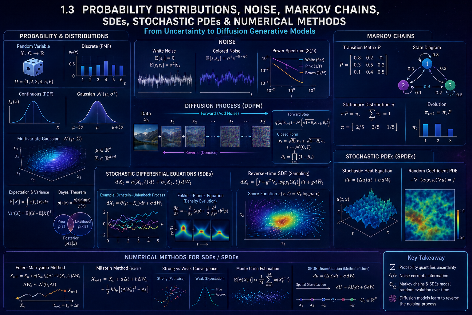
Probability describes uncertainty. Noise corrupts data. Markov chains and SDEs describe how randomness evolves. Diffusion models learn to reverse that evolution.
Source anchors used for this section
- MIT OCW probability material covers distribution functions, common distributions, conditional probability, Bayes’ theorem, joint distributions, law of large numbers, and central limit theorem. (MIT OpenCourseWare)
- MIT statistics notes distinguish discrete probability functions and continuous probability density functions. (MIT OpenCourseWare)
- Stanford CS229 probability review discusses Gaussian random variables and closure properties of multivariate Gaussians. (CS229)
- MIT stochastic-process notes define stochastic processes as collections of random variables indexed by time and introduce Markov chains. (MIT OpenCourseWare)
- MIT Markov-chain notes state existence of stationary distributions for finite-state Markov chains. (MIT OpenCourseWare)
- MIT Itô calculus notes explain that Brownian paths are nowhere differentiable with probability 1, motivating stochastic calculus. (MIT OpenCourseWare)
- Higham’s SIAM Review paper introduces numerical SDE simulation, Euler–Maruyama, Milstein, strong and weak convergence, and stability. (SIAM)
- Gardiner’s Handbook of Stochastic Methods discusses white noise and nonwhite noise processes. (Deutsche Nationalbibliothek)
- Lord, Powell, and Shardlow’s Cambridge text covers stochastic processes, random fields, SDEs, SPDEs, Euler–Maruyama, Milstein, strong/weak approximation, Monte Carlo, and stochastic Galerkin finite-element methods. (Cambridge University Press & Assessment)
- Hairer’s SPDE notes introduce stochastic PDEs through motivating examples including the stochastic heat equation. (hairer.org)
- Ho, Jain, and Abbeel’s DDPM paper defines diffusion probabilistic models as latent-variable models with Gaussian Markov noising and learned reverse denoising. (NeurIPS Proceedings)
- Song et al.’s score-SDE paper formulates generative modeling through forward and reverse stochastic differential equations and connects SDE sampling with probability-flow ODEs. (arXiv)