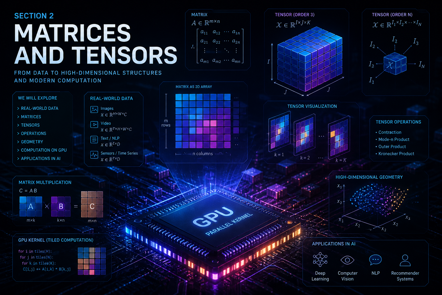
Why matrices and tensors come next
In the previous section, we learned how one object can become a vector.
A house became:
$$ x = \begin{bmatrix} 1200 \\ 3 \\ 2 \\ 10 \\ 3.2 \end{bmatrix} $$This vector represented one house using several features.
But machine learning almost never works with only one object.
Usually, we have many houses, many images, many words, many patients, many time steps, or many training examples. Once we collect many vectors together, we naturally arrive at a matrix.
And once data has more than two directions — for example height, width, and color channels in an image — we naturally arrive at a tensor.
MIT’s 18.06 course describes linear algebra as matrix theory with emphasis on systems of equations, vector spaces, determinants, eigenvalues, and positive definite matrices, all of which are foundational for applied mathematics and AI. (MIT OpenCourseWare)
So the path is:
$$ \text{scalar} \longrightarrow \text{vector} \longrightarrow \text{matrix} \longrightarrow \text{tensor}. $$A scalar is one number.
A vector is a one-dimensional collection of numbers.
A matrix is a two-dimensional collection of numbers.
A tensor, in the machine-learning sense, is a multidimensional array. Kolda and Bader define a tensor as a multidimensional or \(N\)-way array, while also noting the more formal view of an \(N\)-th order tensor as an element of a tensor product of \(N\) vector spaces.
Real-world example 1: a house dataset as a matrix
Suppose we collect data from three houses.
| House | Area | Bedrooms | Floors | Age | Distance | Price |
|---|---|---|---|---|---|---|
| 1 | 1200 | 3 | 2 | 10 | 3.2 | 9.0 |
| 2 | 850 | 2 | 1 | 18 | 8.5 | 6.5 |
| 3 | 1600 | 4 | 2 | 5 | 1.1 | 12.0 |
If price is the target, then the input features are:
$$ X = \begin{bmatrix} 1200 & 3 & 2 & 10 & 3.2 \\ 850 & 2 & 1 & 18 & 8.5 \\ 1600 & 4 & 2 & 5 & 1.1 \end{bmatrix} $$and the target vector is:
$$ y = \begin{bmatrix} 9.0 \\ 6.5 \\ 12.0 \end{bmatrix}. $$Here:
$$ X \in \mathbb{R}^{3 \times 5} $$and:
$$ y \in \mathbb{R}^{3}. $$The matrix \(X\) has:
- 3 rows,
- 5 columns,
- 15 entries.
Each row is one house.
Each column is one feature.
So a matrix lets us store many feature vectors in one object.
In machine learning, this matrix is often called the design matrix.
Real-world example 2: a grayscale image as a matrix
A grayscale image is also naturally represented as a matrix.
Suppose we have a tiny \(4 \times 5\) grayscale image. Each number represents pixel intensity.
$$ I = \begin{bmatrix} 0 & 20 & 50 & 20 & 0 \\ 10 & 80 & 150 & 80 & 10 \\ 20 & 120 & 255 & 120 & 20 \\ 0 & 30 & 60 & 30 & 0 \end{bmatrix} $$Here:
$$ I \in \mathbb{R}^{4 \times 5}. $$The first dimension is height.
The second dimension is width.
The entry \(I_{ij}\) is the brightness of the pixel in row \(i\), column \(j\).
For example:
$$ I_{3,3} = 255 $$is the brightest pixel in this small image.
So a grayscale image is not just a picture. To a model, it is a matrix.
Real-world example 3: a color image as a tensor
A color image has more structure.
Each pixel usually has three color channels:
$$ \text{red},\quad \text{green},\quad \text{blue}. $$So instead of one number per pixel, we have three numbers per pixel.
For a color image with height \(H\), width \(W\), and 3 color channels, we can write:
$$ X \in \mathbb{R}^{H \times W \times 3}. $$This is no longer a matrix.
It has three axes:
- height,
- width,
- color channel.
So it is a third-order tensor.
For a tiny \(2 \times 2\) color image:
$$ X \in \mathbb{R}^{2 \times 2 \times 3}. $$One pixel may be:
$$ X_{1,1,:} {}={} \begin{bmatrix} 255 \\ 0 \\ 0 \end{bmatrix} $$which represents a red pixel.
Another pixel may be:
$$ X_{1,2,:} {}={} \begin{bmatrix} 0 \\ 255 \\ 0 \end{bmatrix} $$which represents a green pixel.
The colon notation means:
keep all values along that axis.
So \(X_{1,1,:}\) means:
row 1, column 1, all color channels.
Real-world example 4: a batch of images as a fourth-order tensor
Deep learning usually processes many examples at once.
Suppose we have a batch of 32 color images.
Each image has size:
$$ 224 \times 224 $$and 3 color channels.
Then the batch may be stored as:
$$ X \in \mathbb{R}^{32 \times 224 \times 224 \times 3}. $$The axes are:
| Axis | Meaning |
|---|---|
| 1 | batch/example index |
| 2 | image height |
| 3 | image width |
| 4 | color channel |
So:
$$ X_{n,i,j,c} $$means:
the value of color channel \(c\) at pixel row \(i\), pixel column \(j\), in image \(n\).
This is a fourth-order tensor.
In PyTorch, images are often stored in another layout:
$$ X \in \mathbb{R}^{32 \times 3 \times 224 \times 224} $$where the axes are:
| Axis | Meaning |
|---|---|
| 1 | batch |
| 2 | channel |
| 3 | height |
| 4 | width |
The mathematics is the same, but the axis order is different.
Real-world example 5: language data as tensors
In natural language processing, a sentence is often converted into a sequence of token embeddings.
Suppose:
- batch size is \(B\),
- sequence length is \(L\),
- embedding dimension is \(d\).
Then the input to a language model layer may be:
$$ X \in \mathbb{R}^{B \times L \times d}. $$For example:
$$ X \in \mathbb{R}^{16 \times 128 \times 768}. $$This means:
- 16 sentences or text chunks,
- 128 tokens per sequence,
- 768 numbers per token embedding.
So one token is a vector:
$$ X_{b,\ell,:} \in \mathbb{R}^{768}. $$One full sentence is a matrix:
$$ X_{b,:,:} \in \mathbb{R}^{128 \times 768}. $$The full batch is a third-order tensor:
$$ X \in \mathbb{R}^{16 \times 128 \times 768}. $$In transformer models, attention scores may have shape:
$$ A \in \mathbb{R}^{B \times H \times L \times L} $$where \(H\) is the number of attention heads.
So modern AI is full of matrices and tensors.
What is a matrix?
A matrix is a rectangular array of numbers.
If a matrix has \(m\) rows and \(n\) columns, we write:
$$ A \in \mathbb{R}^{m \times n}. $$Stanford CS229 uses this notation: \(A \in \mathbb{R}^{m \times n}\) denotes a matrix with \(m\) rows and \(n\) columns, with real-valued entries. (CS229)
A general matrix looks like:
$$ A = \begin{bmatrix} a_{11} & a_{12} & \cdots & a_{1n} \\ a_{21} & a_{22} & \cdots & a_{2n} \\ \vdots & \vdots & \ddots & \vdots \\ a_{m1} & a_{m2} & \cdots & a_{mn} \end{bmatrix}. $$The entry \(a_{ij}\) means:
the entry in row \(i\), column \(j\).
So:
$$ a_{23} $$means:
row 2, column 3.
Matrix shape
The shape of \(A\) is:
$$ m \times n. $$The first number counts rows.
The second number counts columns.
For example:
$$ A = \begin{bmatrix} 1 & 2 & 3 \\ 4 & 5 & 6 \end{bmatrix} $$has 2 rows and 3 columns, so:
$$ A \in \mathbb{R}^{2 \times 3}. $$The entry in row 2, column 3 is:
$$ a_{23} = 6. $$Rows and columns
A matrix can be viewed in two complementary ways.
It can be viewed as a stack of rows:
$$ A = \begin{bmatrix} a_1^\top \\ a_2^\top \\ \vdots \\ a_m^\top \end{bmatrix} $$where each row is a row vector.
It can also be viewed as a collection of columns:
$$ A = \begin{bmatrix} | & | & & | \\ a_1 & a_2 & \cdots & a_n \\ | & | & & | \end{bmatrix} $$where each column is a column vector.
This row-column viewpoint is important because matrix multiplication can be understood using rows, columns, dot products, and linear combinations. Stanford CS229 explicitly describes matrix-vector multiplication both as row inner products and as a linear combination of columns.
Matrix addition
Two matrices can be added only when they have the same shape.
Let:
$$ A = \begin{bmatrix} 1 & 2 \\ 3 & 4 \end{bmatrix} $$and:
$$ B = \begin{bmatrix} 10 & 20 \\ 30 & 40 \end{bmatrix}. $$Then:
$$ A+B = \begin{bmatrix} 1+10 & 2+20 \\ 3+30 & 4+40 \end{bmatrix} {}={} \begin{bmatrix} 11 & 22 \\ 33 & 44 \end{bmatrix}. $$In general, if:
$$ A,B \in \mathbb{R}^{m \times n}, $$then:
$$ (A+B)_{ij} = A_{ij}+B_{ij}. $$But this is not valid:
$$ \mathbb{R}^{2 \times 3} + \mathbb{R}^{3 \times 2}. $$The shapes do not match.
Scalar multiplication of a matrix
A matrix can be multiplied by a scalar.
Let:
$$ A = \begin{bmatrix} 1 & 2 \\ 3 & 4 \end{bmatrix} $$and:
$$ \alpha = 3. $$Then:
$$ \alpha A = 3 \begin{bmatrix} 1 & 2 \\ 3 & 4 \end{bmatrix} {}={} \begin{bmatrix} 3 & 6 \\ 9 & 12 \end{bmatrix}. $$In general:
$$ (\alpha A)_{ij} = \alpha A_{ij}. $$So scalar multiplication scales every entry.
Matrix-vector multiplication
Matrix-vector multiplication is one of the most important operations in AI.
Let:
$$ A = \begin{bmatrix} 1 & 2 & 3 \\ 4 & 5 & 6 \end{bmatrix} $$and:
$$ x = \begin{bmatrix} 10 \\ 20 \\ 30 \end{bmatrix}. $$The shape of \(A\) is:
$$ 2 \times 3. $$The shape of \(x\) is:
$$ 3 \times 1. $$The product (Ax) is valid because the inner dimensions match:
$$ (2 \times 3)(3 \times 1) = 2 \times 1. $$Now compute:
$$ Ax = \begin{bmatrix} 1 & 2 & 3 \\ 4 & 5 & 6 \end{bmatrix} \begin{bmatrix} 10 \\ 20 \\ 30 \end{bmatrix}. $$The first entry is:
$$ 1(10)+2(20)+3(30)=10+40+90=140. $$The second entry is:
$$ 4(10)+5(20)+6(30)=40+100+180=320. $$So:
$$ Ax = \begin{bmatrix} 140 \\ 320 \end{bmatrix}. $$Row-dot-product view
Each output entry is a dot product between one row of \(A\) and the vector \(x\).
The first row of \(A\) is:
$$ \begin{bmatrix} 1 & 2 & 3 \end{bmatrix}. $$The second row is:
$$ \begin{bmatrix} 4 & 5 & 6 \end{bmatrix}. $$So:
$$ Ax = \begin{bmatrix} \text{row}_1(A)\cdot x \\ \text{row}_2(A)\cdot x \end{bmatrix}. $$In general, if:
$$ A \in \mathbb{R}^{m \times n} $$and:
$$ x \in \mathbb{R}^{n}, $$then:
$$ y = Ax \in \mathbb{R}^{m} $$with:
$$ y_i = \sum_{j=1}^{n} A_{ij}x_j. $$Column-linear-combination view
The same product can be viewed another way.
Write \(A\) in columns:
$$ A = \begin{bmatrix} | & | & | \\ a_1 & a_2 & a_3 \\ | & | & | \end{bmatrix}. $$Then:
$$ Ax = x_1a_1+x_2a_2+x_3a_3. $$Using our example:
$$ a_1 = \begin{bmatrix} 1 \\ 4 \end{bmatrix}, \quad a_2 = \begin{bmatrix} 2 \\ 5 \end{bmatrix}, \quad a_3 = \begin{bmatrix} 3 \\ 6 \end{bmatrix}. $$Since:
$$ x = \begin{bmatrix} 10 \\ 20 \\ 30 \end{bmatrix}, $$we get:
$$ Ax = 10 \begin{bmatrix} 1 \\ 4 \end{bmatrix} + 20 \begin{bmatrix} 2 \\ 5 \end{bmatrix} + 30 \begin{bmatrix} 3 \\ 6 \end{bmatrix}. $$So:
$$ Ax = \begin{bmatrix} 10 \\ 40 \end{bmatrix} + \begin{bmatrix} 40 \\ 100 \end{bmatrix} + \begin{bmatrix} 90 \\ 180 \end{bmatrix} {}={} \begin{bmatrix} 140 \\ 320 \end{bmatrix}. $$Matrix-matrix multiplication
Now suppose:
$$ A \in \mathbb{R}^{m \times n} $$and:
$$ B \in \mathbb{R}^{n \times p}. $$Then:
$$ C = AB \in \mathbb{R}^{m \times p}. $$Stanford CS229 defines the matrix product \(C=AB\) entrywise as:
$$ C_{ij} = \sum_{k=1}^{n} A_{ik}B_{kj}, $$with the requirement that the number of columns of \(A\) equals the number of rows of \(B\).
Numerical example
Let:
$$ A = \begin{bmatrix} 1 & 2 & 3 \\ 4 & 5 & 6 \end{bmatrix} $$and:
$$ B = \begin{bmatrix} 1 & 0 \\ 0 & 1 \\ 1 & 1 \end{bmatrix}. $$Then:
$$ A \in \mathbb{R}^{2 \times 3}, \qquad B \in \mathbb{R}^{3 \times 2}. $$So:
$$ AB \in \mathbb{R}^{2 \times 2}. $$Now compute:
$$ AB = \begin{bmatrix} 1 & 2 & 3 \\ 4 & 5 & 6 \end{bmatrix} \begin{bmatrix} 1 & 0 \\ 0 & 1 \\ 1 & 1 \end{bmatrix}. $$The entry in row 1, column 1 is:
$$ 1(1)+2(0)+3(1)=4. $$The entry in row 1, column 2 is:
$$ 1(0)+2(1)+3(1)=5. $$The entry in row 2, column 1 is:
$$ 4(1)+5(0)+6(1)=10. $$The entry in row 2, column 2 is:
$$ 4(0)+5(1)+6(1)=11. $$Therefore:
$$ AB = \begin{bmatrix} 4 & 5 \\ 10 & 11 \end{bmatrix}. $$Matrix multiplication is not usually commutative
In ordinary arithmetic:
$$ 2 \cdot 3 = 3 \cdot 2. $$But matrices do not usually behave this way.
Usually:
$$ AB \neq BA. $$Sometimes (BA) is not even defined.
In the previous example:
$$ A \in \mathbb{R}^{2 \times 3} $$and:
$$ B \in \mathbb{R}^{3 \times 2}. $$So:
$$ AB \in \mathbb{R}^{2 \times 2} $$but:
$$ BA \in \mathbb{R}^{3 \times 3}. $$The shapes are different.
So (AB) and (BA) cannot be equal.
Matrices as linear maps
A matrix is not only a table of numbers.
A matrix can represent a linear transformation.
Let:
$$ A \in \mathbb{R}^{m \times n}. $$Then \(A\) defines a function:
$$ A:\mathbb{R}^{n} \to \mathbb{R}^{m} $$by:
$$ x \mapsto Ax. $$This means:
- the input vector has \(n\) components,
- the output vector has \(m\) components.
For example, let:
$$ A = \begin{bmatrix} 2 & 0 \\ 0 & 1 \end{bmatrix}. $$Then:
$$ A \begin{bmatrix} 3 \\ 4 \end{bmatrix} {}={} \begin{bmatrix} 6 \\ 4 \end{bmatrix}. $$This matrix stretches the first coordinate by a factor of 2 and leaves the second coordinate unchanged.
So a matrix can be understood geometrically.
It transforms space.
Linear maps preserve addition and scalar multiplication
A function \(T:\mathbb{R}^n \to \mathbb{R}^m\) is linear if:
$$ T(u+v)=T(u)+T(v) $$and:
$$ T(\alpha u)=\alpha T(u). $$Matrix multiplication satisfies these properties.
If:
$$ T(x)=Ax, $$then:
$$ T(u+v)=A(u+v)=Au+Av=T(u)+T(v) $$and:
$$ T(\alpha u)=A(\alpha u)=\alpha Au=\alpha T(u). $$Therefore every matrix multiplication map is linear.
This is why matrices are the natural language of linear models.
The identity matrix
The identity matrix is the matrix that does nothing.
For dimension \(n\), it is written:
$$ I_n. $$For example:
$$ I_3 = \begin{bmatrix} 1 & 0 & 0 \\ 0 & 1 & 0 \\ 0 & 0 & 1 \end{bmatrix}. $$For any vector \(x \in \mathbb{R}^3\):
$$ I_3x=x. $$For example:
$$ I_3 \begin{bmatrix} 5 \\ -2 \\ 7 \end{bmatrix} {}={} \begin{bmatrix} 5 \\ -2 \\ 7 \end{bmatrix}. $$The identity matrix plays the same role as the number 1 in ordinary multiplication.
Diagonal matrices
A diagonal matrix has nonzero entries only on the main diagonal.
For example:
$$ D = \begin{bmatrix} 2 & 0 & 0 \\ 0 & 5 & 0 \\ 0 & 0 & -1 \end{bmatrix}. $$Multiplying by \(D\) scales each coordinate separately.
If:
$$ x = \begin{bmatrix} x_1 \\ x_2 \\ x_3 \end{bmatrix}, $$then:
$$ Dx = \begin{bmatrix} 2x_1 \\ 5x_2 \\ -x_3 \end{bmatrix}. $$The Deep Learning book notes that diagonal matrices are computationally efficient because multiplying by a diagonal matrix only scales individual elements.
In machine learning, diagonal matrices appear in:
- feature scaling,
- covariance approximations,
- normalization,
- singular value decomposition,
- optimization preconditioning.
Symmetric matrices
A square matrix is symmetric if:
$$ A = A^\top. $$For example:
$$ A = \begin{bmatrix} 2 & 5 \\ 5 & 3 \end{bmatrix} $$is symmetric.
The entries mirror across the main diagonal.
A distance matrix is often symmetric because the distance from object \(i\) to object \(j\) is usually the same as the distance from object \(j\) to object \(i\). The Deep Learning book gives this as a typical example of symmetry in matrices.
The trace of a matrix
For a square matrix:
$$ A = \begin{bmatrix} a_{11} & a_{12} & \cdots & a_{1n} \\ a_{21} & a_{22} & \cdots & a_{2n} \\ \vdots & \vdots & \ddots & \vdots \\ a_{n1} & a_{n2} & \cdots & a_{nn} \end{bmatrix}, $$the trace is the sum of diagonal entries:
$$ \operatorname{tr}(A)=a_{11}+a_{22}+\cdots+a_{nn}. $$For example:
$$ A = \begin{bmatrix} 2 & 1 \\ 4 & 5 \end{bmatrix}. $$Then:
$$ \operatorname{tr}(A)=2+5=7. $$Trace appears frequently in matrix calculus, optimization, covariance analysis, and neural-network derivations.
Matrix rank
The rank of a matrix measures how many independent directions it contains.
Consider:
$$ A = \begin{bmatrix} 1 & 2 \\ 2 & 4 \end{bmatrix}. $$The second column is twice the first column:
$$ \begin{bmatrix} 2 \\ 4 \end{bmatrix} {}={} 2 \begin{bmatrix} 1 \\ 2 \end{bmatrix}. $$So the two columns do not provide two independent directions.
The rank is:
$$ \operatorname{rank}(A)=1. $$Now consider:
$$ B = \begin{bmatrix} 1 & 2 \\ 3 & 4 \end{bmatrix}. $$The columns are not scalar multiples of each other, so:
$$ \operatorname{rank}(B)=2. $$Stanford’s 2024 CS229 linear algebra review states that column rank is the largest number of linearly independent columns, row rank is the largest number of linearly independent rows, and these are equal, so both are called the rank of the matrix. (CS229)
Column space
The column space of a matrix is the set of all linear combinations of its columns.
If:
$$ A = \begin{bmatrix} | & | & | \\ a_1 & a_2 & a_3 \\ | & | & | \end{bmatrix}, $$then:
$$ \operatorname{Col}(A) {}={} {c_1a_1+c_2a_2+c_3a_3:; c_1,c_2,c_3 \in \mathbb{R}}. $$The column space tells us which outputs are reachable by (Ax).
If:
$$ y = Ax, $$then \(y\) must lie in the column space of \(A\).
This is central in solving linear systems.
Null space
The null space of \(A\) is the set of all vectors that are sent to zero:
$$ \operatorname{Null}(A) {}={} {x:; Ax=0}. $$For example:
$$ A = \begin{bmatrix} 1 & 2 \\ 2 & 4 \end{bmatrix}. $$We want:
$$ Ax=0. $$Let:
$$ x = \begin{bmatrix} x_1 \\ x_2 \end{bmatrix}. $$Then:
$$ \begin{bmatrix} 1 & 2 \\ 2 & 4 \end{bmatrix} \begin{bmatrix} x_1 \\ x_2 \end{bmatrix} {}={} \begin{bmatrix} x_1+2x_2 \\ 2x_1+4x_2 \end{bmatrix} {}={} \begin{bmatrix} 0 \\ 0 \end{bmatrix}. $$The second equation is just twice the first.
So we need:
$$ x_1+2x_2=0. $$Thus:
$$ x_1=-2x_2. $$Let:
$$ x_2=t. $$Then:
$$ x = \begin{bmatrix} -2t \\ t \end{bmatrix} {}={} t \begin{bmatrix} -2 \\ 1 \end{bmatrix}. $$So:
$$ \operatorname{Null}(A) {}={} \operatorname{span} \left{ \begin{bmatrix} -2 \\ 1 \end{bmatrix} \right}. $$The null space tells us which inputs are invisible to the transformation.
Matrix norms
A norm measures size.
For a vector, the Euclidean norm is:
$$ |x|_2 = \sqrt{x_1^2+x_2^2+\cdots+x_n^2}. $$For a matrix, a common norm is the Frobenius norm:
$$ \|A\|_F = \sqrt{\sum_{i,j} A_{ij}^2}. $$For example:
$$ A = \begin{bmatrix} 1 & 2 \\ 3 & 4 \end{bmatrix}. $$Then:
$$ |A|_F = \sqrt{1^2+2^2+3^2+4^2} {}={} \sqrt{30}. $$The Deep Learning book notes that the Frobenius norm is commonly used in deep learning and is analogous to the vector \(L^2\) norm.
Matrix norms are used in:
- regularization,
- stability analysis,
- optimization,
- low-rank approximation,
- neural-network weight control.
Eigenvalues and eigenvectors
For a square matrix \(A\), an eigenvector is a nonzero vector \(v\) such that:
$$ Av = \lambda v. $$Here:
- \(v\) is the eigenvector,
- \(\lambda\) is the eigenvalue.
This equation says:
applying \(A\) to \(v\) only scales \(v\); it does not change its direction.
For example:
$$ A = \begin{bmatrix} 2 & 0 \\ 0 & 3 \end{bmatrix}. $$Then:
$$ A \begin{bmatrix} 1 \\ 0 \end{bmatrix} {}={} \begin{bmatrix} 2 \\ 0 \end{bmatrix} {}={} 2 \begin{bmatrix} 1 \\ 0 \end{bmatrix}. $$So:
$$ v_1 = \begin{bmatrix} 1 \\ 0 \end{bmatrix} $$is an eigenvector with eigenvalue:
$$ \lambda_1 = 2. $$Similarly:
$$ A \begin{bmatrix} 0 \\ 1 \end{bmatrix} {}={} \begin{bmatrix} 0 \\ 3 \end{bmatrix} {}={} 3 \begin{bmatrix} 0 \\ 1 \end{bmatrix}. $$So:
$$ v_2 = \begin{bmatrix} 0 \\ 1 \end{bmatrix} $$is an eigenvector with eigenvalue:
$$ \lambda_2 = 3. $$The Deep Learning book explains eigendecomposition as a way to understand matrices by decomposing them into eigenvectors and eigenvalues.
Singular value decomposition
The singular value decomposition, or SVD, is one of the most important matrix factorizations.
For a matrix:
$$ A \in \mathbb{R}^{m \times n}, $$the SVD writes:
$$ A = U\Sigma V^\top. $$Here:
- \(U\) contains left singular vectors,
- \(\Sigma\) contains singular values,
- \(V\) contains right singular vectors.
The Deep Learning book describes SVD as a factorization of a matrix into singular vectors and singular values, with \(U\) and \(V\) orthogonal and \(\Sigma\) diagonal.
SVD is used in:
- dimensionality reduction,
- principal component analysis,
- low-rank approximation,
- recommendation systems,
- image compression,
- numerical stability,
- understanding neural-network weight matrices.
Matrices in a neural network layer
A fully connected neural-network layer is a matrix operation.
Suppose:
$$ x \in \mathbb{R}^{d} $$is one input vector.
Let:
$$ W \in \mathbb{R}^{d \times h} $$be the weight matrix.
Let:
$$ b \in \mathbb{R}^{h} $$be the bias vector.
Then the layer computes:
$$ z = x^\top W + b. $$If \(x\) is written as a row vector:
$$ x^\top \in \mathbb{R}^{1 \times d}, $$then:
$$ (1 \times d)(d \times h)=1 \times h. $$So:
$$ z \in \mathbb{R}^{h}. $$For a batch:
$$ X \in \mathbb{R}^{n \times d}, $$the layer computes:
$$ Z = XW+b. $$The shape is:
$$ (n \times d)(d \times h)=n \times h. $$So:
$$ Z \in \mathbb{R}^{n \times h}. $$This is the matrix form of many neurons computed at once.
From matrices to tensors
A matrix has two axes.
A tensor may have more than two axes.
Examples:
| Object | Shape | Mathematical type |
|---|---|---|
| scalar | \(()\) | order-0 tensor |
| vector | \((d)\) | order-1 tensor |
| matrix | \((m,n)\) | order-2 tensor |
| grayscale image | \((H,W)\) | order-2 tensor |
| color image | \((H,W,3)\) | order-3 tensor |
| batch of color images | \((N,H,W,3)\) | order-4 tensor |
| video | \((T,H,W,3)\) | order-4 tensor |
| batch of videos | \((N,T,H,W,3)\) | order-5 tensor |
Kolda and Bader state that a first-order tensor is a vector, a second-order tensor is a matrix, and tensors of order three or higher are called higher-order tensors.
Tensor order, modes, and shape
The order of a tensor is the number of axes.
The axes are often called modes.
For example:
$$ X \in \mathbb{R}^{I \times J \times K} $$is a third-order tensor.
It has three modes:
- mode 1 has size \(I\),
- mode 2 has size \(J\),
- mode 3 has size \(K\).
An entry is written:
$$ x_{ijk}. $$This means:
index \(i\) along mode 1, index \(j\) along mode 2, index \(k\) along mode 3.
For an \(N\)-th order tensor:
$$ \mathcal{X} \in \mathbb{R}^{I_1 \times I_2 \times \cdots \times I_N}. $$An entry is:
$$ x_{i_1 i_2 \cdots i_N}. $$The total number of entries is:
$$ I_1 I_2 \cdots I_N. $$A small numerical tensor
Let:
$$ \mathcal{X} \in \mathbb{R}^{2 \times 3 \times 2}. $$This tensor has:
- 2 entries along mode 1,
- 3 entries along mode 2,
- 2 entries along mode 3.
We can display it using two frontal slices.
First slice:
$$ X_{:,:,1} {}={} \begin{bmatrix} 1 & 2 & 3 \\ 4 & 5 & 6 \end{bmatrix}. $$Second slice:
$$ X_{:,:,2} {}={} \begin{bmatrix} 7 & 8 & 9 \\ 10 & 11 & 12 \end{bmatrix}. $$Then:
$$ x_{1,1,1}=1, \qquad x_{2,3,1}=6, \qquad x_{1,2,2}=8, \qquad x_{2,3,2}=12. $$This tensor has:
$$ 2 \cdot 3 \cdot 2 = 12 $$entries.
Tensor slices
A slice is obtained by fixing one index.
For:
$$ \mathcal{X} \in \mathbb{R}^{2 \times 3 \times 2}, $$the slice:
$$ X_{:,:,1} $$fixes the third index at 1.
The slice:
$$ X_{:,:,2} $$fixes the third index at 2.
Each slice is a matrix.
For a color image:
$$ X \in \mathbb{R}^{H \times W \times 3}, $$the red channel is:
$$ X_{:,:,1}. $$The green channel is:
$$ X_{:,:,2}. $$The blue channel is:
$$ X_{:,:,3}. $$So a color image can be seen as three matrices stacked together.
Tensor fibers
A fiber is obtained by fixing all indices except one.
For a third-order tensor:
$$ \mathcal{X} \in \mathbb{R}^{I \times J \times K}, $$examples of fibers are:
$$ \mathcal{X}_{:,j,k}, \qquad \mathcal{X}_{i,:,k}, \qquad \mathcal{X}_{i,j,:}. $$Each fiber is a vector.
In a color image:
$$ X_{i,j,:} $$is the RGB vector at pixel \((i,j)\).
So the pixel itself is a vector.
Tensor unfolding or matricization
Sometimes we convert a tensor into a matrix.
This is called:
- unfolding,
- flattening,
- matricization.
Kolda and Bader describe matricization as the process of reordering the elements of an \(N\)-way array into a matrix and note that the exact ordering convention may vary, as long as it is used consistently.
For:
$$ \mathcal{X} \in \mathbb{R}^{2 \times 3 \times 2}, $$one possible mode-1 unfolding is:
$$ X_{(1)} {}={} \begin{bmatrix} 1 & 2 & 3 & 7 & 8 & 9 \\ 4 & 5 & 6 & 10 & 11 & 12 \end{bmatrix}. $$This gives:
$$ X_{(1)} \in \mathbb{R}^{2 \times 6}. $$One possible mode-2 unfolding is:
$$ X_{(2)} {}={} \begin{bmatrix} 1 & 4 & 7 & 10 \\ 2 & 5 & 8 & 11 \\ 3 & 6 & 9 & 12 \end{bmatrix}. $$This gives:
$$ X_{(2)} \in \mathbb{R}^{3 \times 4}. $$One possible mode-3 unfolding is:
$$ X_{(3)} {}={} \begin{bmatrix} 1 & 2 & 3 & 4 & 5 & 6 \\ 7 & 8 & 9 & 10 & 11 & 12 \end{bmatrix}. $$This gives:
$$ X_{(3)} \in \mathbb{R}^{2 \times 6}. $$Tensor addition and scalar multiplication
Two tensors can be added if they have the same shape.
If:
$$ \mathcal{X},\mathcal{Y} \in \mathbb{R}^{I_1 \times I_2 \times \cdots \times I_N}, $$then:
$$ (\mathcal{X}+\mathcal{Y})_{i_1i_2\cdots i_N} {}={} x_{i_1i_2\cdots i_N} + y_{i_1i_2\cdots i_N}. $$A tensor can also be multiplied by a scalar:
$$ (\alpha \mathcal{X})_{i_1i_2\cdots i_N} {}={} \alpha x_{i_1i_2\cdots i_N}. $$So tensors form vector spaces when their shape is fixed.
For example, all tensors in:
$$ \mathbb{R}^{2 \times 3 \times 2} $$can be added and scaled.
Tensor inner product
If two tensors have the same shape, their inner product is the sum of elementwise products:
$$ \langle \mathcal{X},\mathcal{Y} \rangle {}={} \sum_{i_1=1}^{I_1} \sum_{i_2=1}^{I_2} \cdots \sum_{i_N=1}^{I_N} x_{i_1i_2\cdots i_N} y_{i_1i_2\cdots i_N}. $$For matrices, this becomes:
$$ \langle A,B\rangle {}={} \sum_{i,j} A_{ij}B_{ij}. $$The Frobenius norm of a tensor is:
$$ |\mathcal{X}|_F {}={} \sqrt{ \sum_{i_1=1}^{I_1} \sum_{i_2=1}^{I_2} \cdots \sum_{i_N=1}^{I_N} x_{i_1i_2\cdots i_N}^2 }. $$This generalizes the Euclidean norm of vectors and the Frobenius norm of matrices.
Outer product
The outer product combines vectors to create higher-order objects.
Let:
$$ a = \begin{bmatrix} 1 \\ 2 \end{bmatrix} $$and:
$$ b = \begin{bmatrix} 3 \\ 4 \\ 5 \end{bmatrix}. $$The outer product is:
$$ a \circ b = \begin{bmatrix} 1 \cdot 3 & 1 \cdot 4 & 1 \cdot 5 \\ 2 \cdot 3 & 2 \cdot 4 & 2 \cdot 5 \end{bmatrix} {}={} \begin{bmatrix} 3 & 4 & 5 \\ 6 & 8 & 10 \end{bmatrix}. $$This creates a matrix from two vectors.
Now add a third vector:
$$ c = \begin{bmatrix} 10 \\ 20 \end{bmatrix}. $$Then:
$$ \mathcal{X}=a\circ b\circ c $$is a third-order tensor with entries:
$$ x_{ijk}=a_i b_j c_k. $$For example:
$$ x_{1,2,1}=a_1b_2c_1=1(4)(10)=40. $$And:
$$ x_{2,3,2}=a_2b_3c_2=2(5)(20)=200. $$A tensor formed from the outer product of vectors is called a rank-one tensor.
Tensor rank and CP decomposition
For matrices, rank is the minimum number of rank-one matrices needed to add up to the matrix.
For higher-order tensors, one important idea is similar:
$$ \mathcal{X} \approx \sum_{r=1}^{R} a_r^{(1)} \circ a_r^{(2)} \circ \cdots \circ a_r^{(N)}. $$This is the idea behind CP decomposition, also known as CANDECOMP/PARAFAC.
Kolda and Bader describe CP as decomposing a tensor as a sum of rank-one tensors.
For a third-order tensor:
$$ \mathcal{X} \in \mathbb{R}^{I \times J \times K}, $$a CP decomposition has the form:
$$ \mathcal{X} \approx \sum_{r=1}^{R} a_r \circ b_r \circ c_r. $$Elementwise:
$$ x_{ijk} \approx \sum_{r=1}^{R} a_{ir} b_{jr} c_{kr}. $$This is useful when a large tensor can be approximated by a small number of structured components.
The \(n\)-mode product
A central tensor operation is the \(n\)-mode product.
Let:
$$ \mathcal{X} \in \mathbb{R}^{I_1 \times I_2 \times \cdots \times I_N}. $$Let:
$$ U \in \mathbb{R}^{J \times I_n}. $$Then the \(n\)-mode product is written:
$$ \mathcal{Y} {}={} \mathcal{X} \times_n U. $$The output shape is:
$$ \mathcal{Y} \in \mathbb{R}^{I_1 \times \cdots \times I_{n-1} \times J \times I_{n+1} \times \cdots \times I_N}. $$So the size of mode \(n\) changes from \(I_n\) to \(J\).
Kolda and Bader define the \(n\)-mode matrix product of a tensor with a matrix and give its elementwise formula.
Elementwise:
$$ (\mathcal{X}\times_n U)_{i_1\cdots i_{n-1}j i_{n+1}\cdots i_N} {}={} \sum_{i_n=1}^{I_n} x_{i_1 i_2 \cdots i_N} u_{j i_n}. $$This means:
multiply each mode-\(n\) fiber by the matrix \(U\).
In unfolded form:
$$ Y_{(n)} = U X_{(n)}. $$This connects tensor multiplication back to matrix multiplication.
Tensor contraction
Tensor contraction means summing over one or more shared indices.
The dot product is the simplest contraction:
$$ x^\top y {}={} \sum_{i=1}^{d} x_i y_i. $$Matrix multiplication is also a contraction:
$$ C_{ij} {}={} \sum_{k=1}^{n} A_{ik}B_{kj}. $$The index \(k\) is repeated and summed over.
A tensor contraction generalizes this idea.
For example, suppose:
$$ \mathcal{X} \in \mathbb{R}^{I \times J \times K} $$and:
$$ v \in \mathbb{R}^{K}. $$Then contracting over the third mode gives a matrix:
$$ Y_{ij} {}={} \sum_{k=1}^{K} x_{ijk}v_k. $$So:
$$ Y \in \mathbb{R}^{I \times J}. $$This is exactly what happens when we collapse one tensor dimension by taking weighted sums.
Einstein summation notation
Because tensor formulas can become long, mathematicians and machine-learning libraries often use Einstein summation notation.
Instead of writing:
$$ C_{ij} {}={} \sum_{k=1}^{n} A_{ik}B_{kj}, $$we write:
$$ C_{ij}=A_{ik}B_{kj}. $$The repeated index \(k\) is automatically summed over.
Similarly:
$$ y_i=A_{ij}x_j $$means:
$$ y_i=\sum_j A_{ij}x_j. $$In NumPy, PyTorch, and JAX, this idea appears in functions such as einsum.
For example:
import torch

A = torch.randn(2, 3)
B = torch.randn(3, 4)

C = torch.einsum("ik,kj->ij", A, B)

print(C.shape)
Output:
torch.Size([2, 4])
The notation:
"ik,kj->ij"
means:
- \(A\) has indices \(i,k\),
- \(B\) has indices \(k,j\),
- \(k\) is summed,
- output has indices \(i,j\).
Tucker decomposition
Another major tensor decomposition is the Tucker decomposition.
For a third-order tensor:
$$ \mathcal{X} \in \mathbb{R}^{I \times J \times K}, $$the Tucker decomposition writes:
$$ \mathcal{X} \approx \mathcal{G} \times_1 A \times_2 B \times_3 C. $$Here:
- \(\mathcal{G}\) is the core tensor,
- \(A\), \(B\), and \(C\) are factor matrices,
- each factor matrix acts along one tensor mode.
Kolda and Bader describe Tucker decomposition as a form of higher-order PCA that decomposes a tensor into a core tensor multiplied or transformed by a matrix along each mode.
Elementwise:
$$ x_{ijk} \approx \sum_{p=1}^{P} \sum_{q=1}^{Q} \sum_{r=1}^{R} g_{pqr}a_{ip}b_{jq}c_{kr}. $$For an \(N\)-way tensor:
$$ \mathcal{X} {}={} \mathcal{G} \times_1 A^{(1)} \times_2 A^{(2)} \cdots \times_N A^{(N)}. $$The Tucker decomposition is useful for:
- compression,
- denoising,
- feature extraction,
- dimensionality reduction,
- multilinear PCA,
- multiway data analysis.
Formal mathematical view: tensor products
So far, we have used the machine-learning view:
a tensor is a multidimensional array.
Now we move to the more mathematical view.
Let \(V\) and \(W\) be vector spaces.
The tensor product \(V \otimes W\) is a vector space built from formal products:
$$ v \otimes w, \qquad v \in V,; w \in W. $$These formal products satisfy bilinearity:
$$ (v_1+v_2)\otimes w {}={} v_1\otimes w+v_2\otimes w, $$$$ v\otimes(w_1+w_2) {}={} v\otimes w_1+v\otimes w_2, $$$$ (\alpha v)\otimes w {}={} \alpha(v\otimes w) v\otimes(\alpha w). $$Lerman’s multilinear algebra notes describe two standard ways to think about tensors: as multilinear maps and as elements of tensor products of two or more vector spaces.
The tensor product has a universal property: bilinear maps out of \(V \times W\) correspond to linear maps out of \(V \otimes W\). This is the formal reason tensor products convert bilinear structure into linear structure.
Basis of a tensor product space
Let:
$$ V = \mathbb{R}^{m} $$with basis:
$$ e_1,\dots,e_m. $$Let:
$$ W = \mathbb{R}^{n} $$with basis:
$$ f_1,\dots,f_n. $$Then a basis for:
$$ V \otimes W $$is:
$$ {e_i \otimes f_j:; 1\le i\le m,;1\le j\le n}. $$So:
$$ \dim(V\otimes W)=mn. $$This matches the number of entries in an \(m \times n\) matrix.
That is why a matrix can be viewed as coordinates of an element in a tensor product space.
More generally, if:
$$ V_1,\dots,V_N $$are finite-dimensional vector spaces, then:
$$ V_1 \otimes V_2 \otimes \cdots \otimes V_N $$is the natural space for order-\(N\) tensors.
If:
$$ \dim(V_k)=I_k, $$then:
$$ \dim(V_1 \otimes \cdots \otimes V_N) {}={} I_1I_2\cdots I_N. $$This equals the number of entries in an array of shape:
$$ I_1 \times I_2 \times \cdots \times I_N. $$Tensors as multilinear maps
A multilinear map is a function that is linear in each argument separately.
For example, a bilinear map satisfies:
$$ B(\alpha u_1+\beta u_2,v) {}={} \alpha B(u_1,v)+\beta B(u_2,v) $$and:
$$ B(u,\alpha v_1+\beta v_2) {}={} \alpha B(u,v_1)+\beta B(u,v_2). $$The dot product is bilinear:
$$ \langle u,v\rangle {}={} u^\top v. $$The determinant is multilinear in the columns of a matrix.
Lerman’s notes give the determinant as an example of an \(n\)-linear map when a matrix is viewed as a tuple of column vectors.
In this deeper mathematical view, tensors are not just arrays.
They encode multilinear relationships.
Why matrices are second-order tensors
A vector has one index:
$$ x_i. $$A matrix has two indices:
$$ A_{ij}. $$A third-order tensor has three indices:
$$ x_{ijk}. $$An \(N\)-th order tensor has \(N\) indices:
$$ x_{i_1i_2\cdots i_N}. $$So a matrix is naturally a second-order tensor because it requires two indices to identify one entry.
But in linear algebra, matrices receive special attention because they represent linear maps:
$$ A:\mathbb{R}^{n}\to\mathbb{R}^{m}. $$A general higher-order tensor does not automatically represent a simple linear map from one vector space to another.
Instead, it often represents a multilinear object.
Important distinction: array tensor versus geometric tensor
In machine learning, we often say:
a tensor is a multidimensional array.
This is practical and correct for numerical computing.
But in geometry and physics, tensors must obey transformation rules under changes of coordinates.
Kolda and Bader explicitly warn that the tensor-array notion in tensor decomposition literature should not be confused with tensor fields in physics and engineering.
For this course, we mainly use tensors in the AI sense:
$$ \text{tensor} = \text{structured multidimensional numerical array}. $$But we also keep the deeper mathematical meaning in mind:
$$ \text{tensor} = \text{element of a tensor product space or multilinear map}. $$Both views matter.
Tensors in convolutional neural networks
A convolutional neural network uses tensors everywhere.
Suppose the input batch is:
$$ X \in \mathbb{R}^{N \times C_{\text{in}} \times H \times W}. $$Here:
- \(N\) is batch size,
- \(C_{\text{in}}\) is number of input channels,
- \(H\) is height,
- \(W\) is width.
A convolution kernel may have shape:
$$ K \in \mathbb{R}^{C_{\text{out}} \times C_{\text{in}} \times k_H \times k_W}. $$Here:
- \(C_{\text{out}}\) is number of output channels,
- \(C_{\text{in}}\) is number of input channels,
- \(k_H\) is kernel height,
- \(k_W\) is kernel width.
The output is:
$$ Y \in \mathbb{R}^{N \times C_{\text{out}} \times H' \times W'}. $$A simplified convolution formula is:
$$ Y_{n,c_{\text{out}},i,j} {}={} \sum_{c_{\text{in}}} \sum_{u} \sum_{v} K_{c_{\text{out}},c_{\text{in}},u,v} X_{n,c_{\text{in}},i+u,j+v}. $$This is a tensor contraction.
We multiply kernel entries with input entries and sum over:
- input channels,
- kernel height,
- kernel width.
So convolution is not mysterious.
It is a structured tensor operation.
Tensors in transformer models
Transformers also use tensors heavily.
Suppose:
$$ X \in \mathbb{R}^{B \times L \times d}. $$This is a batch of token embeddings.
Linear projections produce:
$$ Q = XW_Q, \qquad K = XW_K, \qquad V = XW_V. $$For multi-head attention, these are reshaped into:
$$ Q,K,V \in \mathbb{R}^{B \times H \times L \times d_h}. $$The attention score tensor has shape:
$$ S \in \mathbb{R}^{B \times H \times L \times L}. $$One formula is:
$$ S_{b,h,i,j} {}={} \sum_{r=1}^{d_h} Q_{b,h,i,r}K_{b,h,j,r}. $$This means:
for each batch item and each attention head, compare token \(i\) with token \(j\) by taking a dot product over the hidden dimension.
Again, this is a tensor contraction.
The repeated index \(r\) is summed.
The hierarchy of objects
We can now organize the objects clearly.
| Object | Notation | Example shape | Number of indices |
|---|---|---|---|
| scalar | \(x\) | \(()\) | 0 |
| vector | \(x_i\) | \((d)\) | 1 |
| matrix | \(A_{ij}\) | \((m,n)\) | 2 |
| third-order tensor | \(x_{ijk}\) | \((I,J,K)\) | 3 |
| \(N\)-th order tensor | \(x_{i_1\cdots i_N}\) | \((I_1,\dots,I_N)\) | \(N\) |
The key idea is:
each additional axis adds one more index.
Why tensors matter in AI
Tensors matter because AI data is naturally multi-axis.
Images have:
$$ \text{height} \times \text{width} \times \text{channels}. $$Videos have:
$$ \text{time} \times \text{height} \times \text{width} \times \text{channels}. $$Text batches have:
$$ \text{batch} \times \text{sequence} \times \text{embedding}. $$Attention has:
$$ \text{batch} \times \text{heads} \times \text{query positions} \times \text{key positions}. $$Convolution kernels have:
$$ \text{output channels} \times \text{input channels} \times \text{kernel height} \times \text{kernel width}. $$So tensors are not optional in deep learning.
They are the native format of modern AI computation.
Common mistakes
Mistake 1: Calling every array a matrix
A matrix has exactly two axes.
A color image:
$$ X \in \mathbb{R}^{H \times W \times 3} $$is not a matrix.
It is a third-order tensor.
Mistake 2: Ignoring axis meaning
The shape:
$$ (32,224,224,3) $$means something different from:
$$ (32,3,224,224). $$The numbers are the same, but the axis meanings are different.
Mistake 3: Confusing matrix multiplication with elementwise multiplication
Matrix multiplication:
$$ C_{ij}=\sum_k A_{ik}B_{kj} $$is not the same as elementwise multiplication:
$$ C_{ij}=A_{ij}B_{ij}. $$In Python, these are usually different operations.
For example, in NumPy:
A @ B       # matrix multiplication
A * B       # elementwise multiplication
Mistake 4: Forgetting batch dimensions
A single image may have shape:
(224, 224, 3)
A batch of images may have shape:
(32, 224, 224, 3)
The extra dimension is the batch dimension.
Many deep learning errors come from forgetting whether the batch axis is present.
Mistake 5: Thinking tensors are always deep and abstract
In machine learning, a tensor can be very practical.
A tensor may simply be:
- a batch of images,
- a batch of embeddings,
- a stack of time-series measurements,
- a collection of attention scores.
The abstract mathematics becomes useful because it gives us a precise language for these objects.
Section summary
A matrix is a two-dimensional array:
$$ A \in \mathbb{R}^{m \times n}. $$Its entries are:
$$ A_{ij}. $$A matrix can represent:
- a data table,
- a grayscale image,
- a system of equations,
- a linear transformation,
- a neural-network weight layer.
Matrix-vector multiplication is:
$$ y=Ax, $$with:
$$ y_i=\sum_j A_{ij}x_j. $$Matrix-matrix multiplication is:
$$ C=AB, $$with:
$$ C_{ij}=\sum_k A_{ik}B_{kj}. $$A tensor generalizes vectors and matrices to more axes:
$$ \mathcal{X} \in \mathbb{R}^{I_1 \times I_2 \times \cdots \times I_N}. $$Its entries are:
$$ x_{i_1i_2\cdots i_N}. $$A vector is a first-order tensor.
A matrix is a second-order tensor.
A color image is often a third-order tensor.
A batch of color images is often a fourth-order tensor.
A tensor can be sliced, unfolded, contracted, multiplied along modes, and decomposed.
The \(n\)-mode product is:
$$ \mathcal{Y} {}={} \mathcal{X} \times_n U. $$The CP decomposition writes a tensor approximately as a sum of rank-one tensors:
$$ \mathcal{X} \approx \sum_{r=1}^{R} a_r^{(1)} \circ a_r^{(2)} \circ \cdots \circ a_r^{(N)}. $$The Tucker decomposition writes:
$$ \mathcal{X} \approx \mathcal{G} \times_1 A^{(1)} \times_2 A^{(2)} \cdots \times_N A^{(N)}. $$At the deeper mathematical level, tensors can be understood as elements of tensor product spaces or as multilinear maps.
So the conceptual path is:
$$ \text{numbers} \to \text{vectors} \to \text{matrices} \to \text{tensors} \to \text{multilinear computation}. $$And this is exactly the path modern AI follows.
Source anchors used for this section
- MIT OCW 18.06 identifies linear algebra as matrix theory with applications to systems of equations, vector spaces, determinants, eigenvalues, similarity, and positive definite matrices. (MIT OpenCourseWare)
- Stanford CS229 linear algebra notes define matrix notation, row/column notation, and matrix multiplication using the entrywise summation formula. (CS229)
- Boyd & Vandenberghe’s Introduction to Applied Linear Algebra explicitly connects vectors, matrices, least squares, data fitting, machine learning, AI, image processing, and other applied areas.
- Goodfellow, Bengio, and Courville’s Deep Learning discusses Frobenius norms, diagonal matrices, symmetric matrices, orthogonal matrices, eigendecomposition, and SVD in a deep-learning linear algebra chapter.
- Kolda & Bader’s SIAM Review paper defines tensors as multidimensional or \(N\)-way arrays, distinguishes first-order vectors and second-order matrices, defines tensor unfolding/matricization, \(n\)-mode products, CP decomposition, and Tucker decomposition.
- Multilinear algebra notes by Lerman and LMU notes give the formal tensor-product and multilinear-map view, including the universal property of tensor products.